Conditional Formatting - Highlighting Rows with Matching Cells in Multiple Columns

[ScottTemple]

Hello,

I would like to highlight an entire row using Conditional Formatting, when multiple cells in a row match, but across three columns. In the below example, only the last two rows would highlight as they have multiple matches in all three columns.

 

[awoohaw]

You can try this:

Book1
	D	E	F	G	H	I
1		Work Order	Coil #	Coil Wt		Building CF Formula
2
3		500546	13	441		2
4		500546	15	441		2
5		789243	12	127		0
6		483541	22	289		3
7		483541	22	289		3
8
Sheet3

Cell Formulas
Range	Formula
I3:I7	I3	=(SUM(--($E3=$E$3:$E$7))>1)+ (SUM(--($F3=$F$3:$F$7))>1) +(SUM(--($G3=$G$3:$G$7))>1)

Cells with Conditional Formatting
Cell	Condition		Cell Format	Stop If True
E3:G7	Expression	=(SUM(--($E3=$E$3:$E$7))>1)+ (SUM(--($F3=$F$3:$F$7))>1) +(SUM(--($G3=$G$3:$G$7))>1)	text	NO

 

[ScottTemple]

Thanks awoohaw, is it possible without adding a new column though?

 

[awoohaw]

Thanks awoohaw, is it possible without adding a new column though?

The new column is not necessary. That is how I built the CF formula. I build formulas to result in TRUE, and then paste into the CF dialog.

 

[ScottTemple]

The new column is not necessary. That is how I built the CF formula. I build formulas to result in TRUE, and then paste into the CF dialog.

Ah gotcha. I'm not able to get the CF to work though. To confirm in the 'Apply to range' I'm inputting the entire column range for E, F, G (E1:G2460) and then I select Formula for the 'Rule Type' and enter in your formula of

=(SUM(--($E3=$E$3:$E$7))>1)+ (SUM(--($F3=$F$3:$F$7))>1) +(SUM(--($G3=$G$3:$G$7))>1)

 

[awoohaw]

copy from edit mode the entire formula (including the = sign) in cell I3. Escape out of edit mode.
Then select cell E3. From Home, select Conditional Formatting.
Click New Rule, From a Formula
Paste the formula from I3 into the format values bar.
Select your formatting. Click OK.

Then use paste special (or format painter) to conditionally format the rest of the range.

 

[ScottTemple]

Sorry what edit mode are you referring to? The CF formula is working, but it is highlighting every row, not just those that have all three in common.

 

[awoohaw]

When press F2 to change a cell formula, you are in edit mode in that cell.

ONLY PUT CF in one cell FIRST (THE TOP LEFT CELL). Then copy formatting. Do not mess around with the "apply to" button.

To figure out why the formatting isn't working...


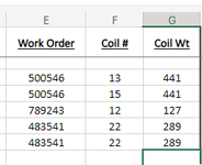
Copy the mini workbook I have done onto a fresh worksheet.
And perform the CF steps below first before applying them to your workbook.

Put the formula that I have in cell I3 which is:
=(SUM(--($E3=$E$3:$E$7))>1)+ (SUM(--($F3=$F$3:$F$7))>1) +(SUM(--($G3=$G$3:$G$7))>1)
(DO NOT CHANGE the mixed absolute references of the formulas).

into your clipboard:
1. select cell I3
2. Press F2
3. Select the entire formula.
4. Click any of:

a. the copy icon on ribbon,​

b. Right click and click copy​

c. CNTL-C keystroke​

5. Exit out of that cell (press Esc)
6. Select ONLY cell E3
7. From HOME ribbon select Conditional Formatting
9. Click New Rule
10 Click Use a Formula to Determine Which Cells to Format
11. In the white box paste the formula you copied to clip board, by

a. click the paste icon​

b. right click and paste​

c. CNTL-V​

12. Click Format
13. Choose your formatting
14. Click OK
15. Copy the format of cell E3 to the rest of your range.


If you still can't figure it out. Please use the xl2bb add in and paste a mini worksheet of that section of your workbook.
Please include the top left cell of your worksheet that has a conditional formatting formula in it.
And be sure to click the checkbox to include conditional formatting rules so the forum can see that as well.

 

[ScottTemple]

I appreciate the breakdown, but I'm familiar with how to input formulas, I've just never heard of using F2 to enter Edit mode, normally you just type the formula in the cell. I've provided a snapshot of the CF in action, and it should only highlight the last two cells, as column E, F, G all match, but it's highlighting all except row 7 for some reason, when it should just be rows 6 and 7.

 

[awoohaw]

I really needed you to post an xl2bb so I can see what cells the CF applies to in the application.
You did not say how you copied the CF throughout the rest of the worksheet.