ajwooden32
New Member
- Joined
- Feb 5, 2024
- Messages
- 11
- Office Version
- 365
- Platform
- Windows
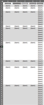
Is there a way to conditional format every other sets of multiple rows based off if a cell in the 1st column has text in it? The text in column A varies so formatting off specific text would require multiple rules.
Below is a manual, created image of what I'm looking for.

Below is a manual, created image of what I'm looking for.