Good Mooring Joe4, My company won't allow me to use your XL2BB tool. I am trying to get our IT department to come to this site with me so they can see that it isn't something questionable.
I can upload a snapshot of my pivot table with a small data set. I will explain clearly.
I am already noticing issues using a Pivot Table for this type of analysis. I may have to use INDEX/MATCH or SUMIF instead. But for now, I just need a conditional formatting for 3 conditions across columns if these conditions are met.
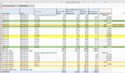
PIVOT TABLE COLUMNS: A thru G. Columns D, E, and F are just three different types of benefits. Not everyone elected all three.
Med, Dental, Vision. Some have 1 or 2 or 3 elections.
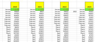
VLOOKUP IN COLUMN H: This formula is looking at column C of the PT and also at another tab that lists ONLY FRIDAY dates for the year 2020 thru future years.
An #N/A result in column G means that the date in the PT is
NOT a Friday.
The pivot table data grows when new data is added to the source tab - weekly or monthly.
This data reflects benefits costs that were deducted from each employee's PR check. I set this up to track if there were any weeks missed (did HR miss deducting benefits costs from anyone on FRIDAY.
I NEED CONDITIONAL FORMATTINGS FOR THE FOLLOWING: COLOR CODING TO GO FROM COLUMN A THRU H IF THE FOLLOWING IS TRUE
HIGHLIGHT ORANGE: For example, If HR posted a deduction with with a NON FRIDAY DATE - and there IS a total greater or lesser than ZERO in column G - that means that the deduction (or deductions) were technically NOT missed. The deduction just wasn't posted with a FRIDAY date.
HIGHLIGHT GREEN: For example, If HR posted a deduction with a NON FRIDAY DATE and the total is zero in column G - that means that the deduction was MISSED completely.
HIGHLIGHT YELLOW: For example, If HR posted a deduction WITH A FRIDAY DATE and the total is zero in column G - that means that no amount for the the deduction was actually made.
MISSED and needs to be researched.
I've color coded the pivot table so you can see how the results should be. This pivot has approx 100 employee names but my snapshot is for just two. Conditional Formatting starts over at name change in column A. I hope that is helpful.
Here is my formula in Column H that is looking the the tab with Friday dates listed, in case you need to see it.
Excel Formula:
=IF(YEAR(C5)=2020,VLOOKUP(C5,CALENDAR!F:F,1,0),
IF(YEAR(C5)=2021,VLOOKUP(C5,CALENDAR!I:I,1,0),
IF(YEAR(C5)=2022,VLOOKUP(C5,CALENDAR!L:L,1,0),
IF(YEAR(C5)=2023,VLOOKUP(C5,CALENDAR!N:N,1,0)))))
Afterwards, could you please direct me to a link where I can take a course for learning complex CF's? I really need to become self-sufficient in this. Thank you so much!
")