Conditional Formatting with Outlier Values

[yankeez245]

Hello,

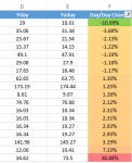
I have the following list of values and the conditional formatting of the values in column F is being thrown off because of the three outlier values I have (38.88%, 7.33%, -10.99%). The non-outlier values are all in the medium shade of orange because Excel thinks the range of numbers is between -10.99% and 38.88%, but the actual range of numbers is between -3.68% and 3.29%. The attached screenshot is the top ten most negative and positive values out of the entire list, which contains over 2000 numbers.

Is there a way to make it so that any value greater than 3% is dark red, less than 3% is dark green, and everything else is adjusted as if the max values in the list are -3% and 3%?

Thank you.

 

[Fluff]

Is this what you want

+Fluff New.xlsm
	F
1
2	-10.99%
3	-3.68%
4	-2.13%
5	-1.22%
6	-1.19%
7	-1.18%
8	-1.17%
9	1.10%
10	1.25%
11	1.26%
12	2.12%
13	2.31%
14	2.31%
15	2.93%
16	2.93%
17	3.29%
18	7.33%
19	38.88%
20
Data2

Cells with Conditional Formatting
Cell	Condition		Cell Format	Stop If True
F2:F21	Other Type	Color scale		NO

Both 2.93% values are dark red, but for some reason, are not being picked up by XL2BB

 

[yankeez245]

Hi thanks for your response. Yes, that is basically what I want, except the 1.10-1.26% should be light green. There are roughly 2000 values between -1% and 1% in the sheet that I attached, so I would want all of those to be various shades of yellow.

How did you get that formatting?

I appreciate your help. Thanks

 

[Fluff]

If you edit the rule & change Minimum to Number with -.03 & change Max to Number & use .03