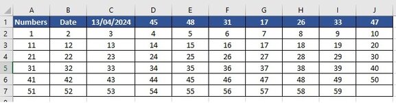
so you want the cells in A2 to J7
to format as yellow - if the cell is = to any number on D1 to J1
setup a rule
=countif($D$1:$J$1,A2)>0
for 2007, 2010 , 2013 , 2016 , 2019 or 365 Subscription excel version
Conditional Formatting
Highlight applicable range >>
A2:J7 - Change, reduce or extend the rows to meet your data range of rows
Home Tab >> Styles >> Conditional Formatting
New Rule >> Use a formula to determine which cells to format
Edit the Rule Description: Format values where this formula is true:
=countif($D$1:$J$1,A2)>0
Format [Number, Font, Border, Fill]
choose the format you would like to apply when the condition is true
OK >> OK
| Book2 |
|---|
|
|---|
| A | B | C | D | E | F | G | H | I | J |
|---|
| 1 | | | | 1 | 2 | 3 | 4 | 5 | 6 | 7 |
|---|
| 2 | 1 | 4 | 7 | 10 | 13 | 16 | 19 | 6 | 25 | 7 |
|---|
| 3 | 15 | 2 | 2 | 4 | -2.5 | -5.8 | -9.1 | -12.4 | -15.7 | -19 |
|---|
| 4 | 15 | 2 | 2 | 4 | -2.5 | -5.8 | 7 | -12.4 | 7 | -19 |
|---|
| 5 | 15 | 2 | 2 | 4 | -2.5 | -5.8 | -9.1 | -12.4 | -15.7 | -19 |
|---|
| 6 | 15 | 2 | 2 | 4 | -2.5 | 5 | -9.1 | -12.4 | 5 | -19 |
|---|
| 7 | 15 | 2 | 2 | 4 | -2.5 | -5.8 | -9.1 | -12.4 | -15.7 | -19 |
|---|
|
|---|