Conditional Formatting

[Frank Harrison]

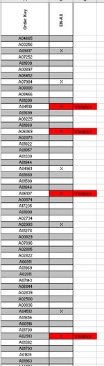
I am looking to use conditional formatting to highlight a cell when a one in five rows condition is exceeded.

Order Key	VS-455
A04532	X
A01323
A01022
A01331
A06877	X Thid cell should highligrt red because there is an "X" Four rows above
A01003
A01922
A02403
A02740
A04565	X
A01394
A01246
A07754
A01271
A09886	X

 

[Joe4]

You should be able to use a COUNTIF to count how many "X"s there are in the 4 rows above, and if it is more than 0, i.e. the Conditional Formatting formula would start in B6 and look like:

=COUNTIF(B2:B5,"X")>0

 

[Frank Harrison]

Every time an "X" occurs I need it to evaluate the four cell above and below to make sure no othes rows contain an "X"

 

[Joe4]

OK, looks you conditions changed, as you now want to check above AN D below, instead of just below.

What row/column does your data actually start in?

 

[Frank Harrison]

Sample file attached I think the rows above would nohave to be considered because they would be covered.

 

[Joe4]

What row/column does your data actually start in?

You did not answer my question, and your image does not show row or column headers, so I cannot see what ranges you are working with.

 

[Frank Harrison]

 

[Joe4]

Sorry, I was out of town for a few days and just getting back now.

Your image does not seem to match you last description, in which you said:

Every time an "X" occurs I need it to evaluate the four cell above and below to make sure no othes rows contain an "X"

Your image suggest it is only looking one way, and not both, or else lines 9 and 23 would also be highlighted.

If your image is accurate (and your last description is not), then if you select B6 to the end of your range, you can then use this Conditional Formatting formula:

=AND(B6="X",COUNTIF(B2:B5,"X")>0)

You would need to use slightly adjusted formula for cells B3:B5, i.e.

for cell B3:

=AND(B3="X",B2="X")>0)

for cell B4:

=AND(B4="X",COUNTIF(B2:B3,"X")>0)

for cell B5:

=AND(B5="X",COUNTIF(B2:B4,"X")>0)