Conditional INDEX-MATCH statement involving three data categories

[DaRook1e]

Dear community,

I've been struggling a lot lately with the following task but so far in vain... I am not a regular in excel forums bt in this case I don't have any alternative. Basically, I am trying to figure out how to distinguish between repeating categories in groups 2 and 3 while groups 1 remains unique. My result should then either multiply the values of matched categories or return the single values from the unmatched categories. I have been trying really hard with combinations using INDEX, MATCH, IF and COUNTIF statements but without success. Please read below and refer to the attached screenshot for more clarity.

IF:
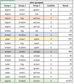
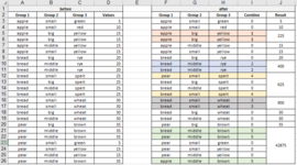
Items in group 1 differ from each other (unique values) but items in group 2 and 3 are the same. In this case multiply the values in column "D" of the matching rows with each other.

ELSE:
return the row from table "before"

Result should match the one in column "J".

Your help will be very much appreciated! Thank you in advance.

Best
Evgeni

 

[C Moore]

I can't figure out your values, but it sounds like you need sumproduct with criteria.

 

[KRice]

Why are the values in rows 13 & 14 multiplied together when there is a Group 2 mismatch? A similar question for rows 23, 24, and 25 where there are mismatches in Groups 2 & 3.

What version of Excel are you using?

If you have Excel 365, is this what you want?

MrExcel_20220505B.xlsx
	A	B	C	D	E	F	G
1
2	Group 1	Group 2	Group 3	Values		Post #1 Result	My Result
3	apple	small	green	5		5	5
4	apple	small	red	10		10	10
5	apple	big	yellow	15		225	225
6	apple	big	yellow	15		225	225
7	apple	middle	yellow	15		15	15
8	apple	small	yellow	15		15	15
9	bread	big	rye	20		20	20
10	bread	middle	rye	20		400	400
11	bread	middle	rye	20		400	400
12	bread	small	spelt	25		625	625
13	bread	big	spelt	25		625	25
14	bread	middle	spelt	25		625	25
15	bread	small	spelt	25		625	625
16	bread	small	wheat	30		900	900
17	bread	small	wheat	30		900	900
18	bread	big	wheat	30		30	30
19	bread	middle	wheat	30		30	30
20	pear	big	brown	35		35	35
21	pear	middle	brown	35		42875	42875
22	pear	middle	brown	35		42875	42875
23	pear	small	green	5		42875	5
24	pear	small	yellow	15		42875	15
25	pear	middle	yellow	15		42875	15
26	pear	middle	brown	35		42875	42875
Sheet8

Cell Formulas
Range	Formula
G3:G26	G3	=PRODUCT(FILTER($D$3:$D$26,($A$3:$A$26=$A3)*($B$3:$B$26=$B3)*($C$3:$C$26=$C3)))

 

[KRice]

Or a non-365 version:

MrExcel_20220505B.xlsx
	A	B	C	D	E	F	G	H
2	Group 1	Group 2	Group 3	Values		Post #1 Result	My Result	Non Excel 365
3	apple	small	green	5		5	5	5
4	apple	small	red	10		10	10	10
5	apple	big	yellow	15		225	225	225
6	apple	big	yellow	15		225	225	225
7	apple	middle	yellow	15		15	15	15
8	apple	small	yellow	15		15	15	15
9	bread	big	rye	20		20	20	20
10	bread	middle	rye	20		400	400	400
11	bread	middle	rye	20		400	400	400
12	bread	small	spelt	25		625	625	625
13	bread	big	spelt	25		625	25	25
14	bread	middle	spelt	25		625	25	25
15	bread	small	spelt	25		625	625	625
16	bread	small	wheat	30		900	900	900
17	bread	small	wheat	30		900	900	900
18	bread	big	wheat	30		30	30	30
19	bread	middle	wheat	30		30	30	30
20	pear	big	brown	35		35	35	35
21	pear	middle	brown	35		42875	42875	42875
22	pear	middle	brown	35		42875	42875	42875
23	pear	small	green	5		42875	5	5
24	pear	small	yellow	15		42875	15	15
25	pear	middle	yellow	15		42875	15	15
26	pear	middle	brown	35		42875	42875	42875
Sheet8

Cell Formulas
Range	Formula
G3:G26	G3	=PRODUCT(FILTER($D$3:$D$26,($A$3:$A$26=$A3)*($B$3:$B$26=$B3)*($C$3:$C$26=$C3)))
H3:H26	H3	=PRODUCT(IFERROR(($D$3:$D$26)/(($A$3:$A$26=$A3)*($B$3:$B$26=$B3)*($C$3:$C$26=$C3)),""))

 

[DaRook1e]

Or a non-365 version:

MrExcel_20220505B.xlsx
	A	B	C	D	E	F	G	H
2	Group 1	Group 2	Group 3	Values		Post #1 Result	My Result	Non Excel 365
3	apple	small	green	5		5	5	5
4	apple	small	red	10		10	10	10
5	apple	big	yellow	15		225	225	225
6	apple	big	yellow	15		225	225	225
7	apple	middle	yellow	15		15	15	15
8	apple	small	yellow	15		15	15	15
9	bread	big	rye	20		20	20	20
10	bread	middle	rye	20		400	400	400
11	bread	middle	rye	20		400	400	400
12	bread	small	spelt	25		625	625	625
13	bread	big	spelt	25		625	25	25
14	bread	middle	spelt	25		625	25	25
15	bread	small	spelt	25		625	625	625
16	bread	small	wheat	30		900	900	900
17	bread	small	wheat	30		900	900	900
18	bread	big	wheat	30		30	30	30
19	bread	middle	wheat	30		30	30	30
20	pear	big	brown	35		35	35	35
21	pear	middle	brown	35		42875	42875	42875
22	pear	middle	brown	35		42875	42875	42875
23	pear	small	green	5		42875	5	5
24	pear	small	yellow	15		42875	15	15
25	pear	middle	yellow	15		42875	15	15
26	pear	middle	brown	35		42875	42875	42875
Sheet8

Cell Formulas
Range	Formula
G3:G26	G3	=PRODUCT(FILTER($D$3:$D$26,($A$3:$A$26=$A3)*($B$3:$B$26=$B3)*($C$3:$C$26=$C3)))
H3:H26	H3	=PRODUCT(IFERROR(($D$3:$D$26)/(($A$3:$A$26=$A3)*($B$3:$B$26=$B3)*($C$3:$C$26=$C3)),""))

Hey KRice,

much appreciated, works perfectly! Apologies for the misunderstanding: I multiplied only the coloured rows because they were matches. I merged the cells and it looked like the uncoloured cells were also part of the output, when in fact they weren't. I prepared an Excel but I couldn't upload it and had to attach the screenshot as on my working laptop I am not allowed to install xl2bb.

Now, whereas this solves the better part of my task, I would like to optimize the output and see only the grouped results. This means that I have to exclude duplicate outputs, e.g. apple>big>yellow should be displayed only once, the other row should be excluded. This is needed because this new table with the output is the input for further calculations down the road. I don't see a way to this in excel but in VBA should be no problem. What do you think, how could this problem be solved in the best way?

Best
Evgeni

 

[KRice]

Give this a try...

MrExcel_20220505B.xlsx
	A	B	C	D	E	F	G	H	I
2	Group 1	Group 2	Group 3	Values		Post #1 Result	My Result	Non Excel 365	Non Excel 365 & check for prior match
3	apple	small	green	5		5	5	5	5
4	apple	small	red	10		10	10	10	10
5	apple	big	yellow	15		225	225	225	225
6	apple	big	yellow	15		225	225	225
7	apple	middle	yellow	15		15	15	15	15
8	apple	small	yellow	15		15	15	15	15
9	bread	big	rye	20		20	20	20	20
10	bread	middle	rye	20		400	400	400	400
11	bread	middle	rye	20		400	400	400
12	bread	small	spelt	25		625	625	625	625
13	bread	big	spelt	25		625	25	25	25
14	bread	middle	spelt	25		625	25	25	25
15	bread	small	spelt	25		625	625	625
16	bread	small	wheat	30		900	900	900	900
17	bread	small	wheat	30		900	900	900
18	bread	big	wheat	30		30	30	30	30
19	bread	middle	wheat	30		30	30	30	30
20	pear	big	brown	35		35	35	35	35
21	pear	middle	brown	35		42875	42875	42875	42875
22	pear	middle	brown	35		42875	42875	42875
23	pear	small	green	5		42875	5	5	5
24	pear	small	yellow	15		42875	15	15	15
25	pear	middle	yellow	15		42875	15	15	15
26	pear	middle	brown	35		42875	42875	42875
Sheet8

Cell Formulas
Range	Formula
G3:G26	G3	=PRODUCT(FILTER($D$3:$D$26,($A$3:$A$26=$A3)*($B$3:$B$26=$B3)*($C$3:$C$26=$C3)))
H3:H26	H3	=PRODUCT(IFERROR(($D$3:$D$26)/(($A$3:$A$26=$A3)*($B$3:$B$26=$B3)*($C$3:$C$26=$C3)),""))
I3:I26	I3	=IF(SUMPRODUCT(($A$2:$A2=$A3)*($B$2:$B2=$B3)*($C$2:$C2=$C3))>0,"",PRODUCT(IFERROR(($D$3:$D$26)/(($A$3:$A$26=$A3)*($B$3:$B$26=$B3)*($C$3:$C$26=$C3)),"")))

 

[DaRook1e]

Awesome work! KRice, you saved me tons of time, much appreciated!
P.S. I use Office 365, sorry for overlooking your question before...

 

[KRice]

I'm happy to help, and thanks for letting me know. You should update your account details to indicate you use Excel 365, as solutions offered can, and often do, depend on whether the enhanced functions in 365 are available.

 

[DaRook1e]

Thanks for the heads-up, it's done now.
Best,
Evgeni

 

[KRice]

Thanks!