Conditional Loop - Copy Paste to new Workbook

[FrankieG]

Dear All,

First of all thanks for your help in advance.

I have a complicated excel model to make projections for the future. These projections are contingent on many inputs, and as such I am using a single input cell (or actually two) to pull in all the related inputs at the same time per person.

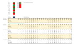
In the example enclosed these inputs are provided in cells C25 and C26. For simplicity I have named them Person 1, Person 2 (and the n=500) whilst there are also different scenarios per person possible (scenario 1-10).

Depending on the combination in cell C25 and C26 a certain table with results is produced, do note that this table is pretty extensive in itself with roughly 100 rows x 100 columns.

It is not required to run all persons and all scenarios all the time, and hence there is an YES/NO switch per person and a YES/NO switch per scenario. Only the activated combinations matter.

I am trying to find a way to:
1. Run all relevant selected combinations of cells C25 and C26 (in this example: Person 1 & Scenario 1, Person 1 & Scenario 3, Person 5 & Scenario 1, Person 5 & Scenario 3 etc). This is a lot of combinations, whilst excluding the combinations that are not selected is equally important to save computing power.
2. Create a new workbook
3. Copy paste all results next to each other to this new workbook. Note that all relevant results per person/per scenario are captured in a single table.

So in short: want to change nothing to the model as-is, with the exception to run a loop for all possible scenarios, and create a new workbook to store these results in one go.

Regards
FG

 

[offthelip]

You haven't given any details about which columns your results are in or exactly which columns you Person and Scenarios are so I have had to guess but try this:

Sub test()
Dim outarr
cols = 30
' Assume 7 rows for each result and columns 1 to 30 ( A to AD)
parr = Range("b2:C21")
sarr = Range("d2:E11")
ReDim outarr(1 To (UBound(parr, 1) * UBound(sarr, 1) * 7), 1 To cols) As Variant
indi = 0
For i = 1 To UBound(parr, 1) ' Persons loop
  If parr(i, 2) = "Yes" Then
    For j = 1 To UBound(sarr, 1) ' scenario loop
     If sarr(j, 2) = "Yes" Then
        Range("c25") = parr(i, 1)
        Range("C26") = sarr(j, 1)
        temparr = Range("A28:ad34")  ' pick up results Note yo didn't say where they were!!
        For k = 1 To 7               ' copy results to output buffer
         For kk = 1 To cols
          outarr(indi + k, kk) = temparr(k, kk)
         Next kk
        Next k
        indi = indi + 7
     End If
    Next j
 End If
Next i
Workbooks.Add
Range(Cells(1, 1), Cells(indi + 7, 30)) = outarr

End Sub

I have assumes the persons are in B2 to C21
Scenarios in D2 to E11
Results in A28 to AD34

 

[FrankieG]

Offthelip - thank you very much. Really do appreciate your help here.

1. On the location of the Persons and Scenarios names: these are name ranges / arrays. Is the location of the referenced cell still relevant or is it possible to reference these name ranges altogether e.g. range name "Persons.Selected" and "Scenarios.Selected"?

Also on the location of the result copy paste, since they are in a new workbook I am not too worried about the location. But since we are talking about a lot of different results (hundreds of copy pastes potentially) there would probably a sort of offset function required as I would need the results one below the other.

Best
FG

 

[offthelip]

If you are using named ranges for the persons and scenarios then instead of the code:

parr = Range("b2:C21")
sarr = Range("d2:E11")

you can use

parr = Range("Persons")
sarr = Range("Scenarios")

Assuming the named ranges are "Persons" and "Scenarios"

Also on the location of the result copy paste, since they are in a new workbook I am not too worried about the location. But since we are talking about a lot of different results (hundreds of copy pastes potentially) there would probably a sort of offset function required as I would need the results one below the other.

I don't understand this since comment: the code I have written does exactly this.
It doesn't use copy and paste because that is very very slow, it copies all the results into an output variant array ( output buffer) and then writes the variant array to the new workbook. ( This is the last 2 lines of the code, it takes longer to explain than the code!!)
You haven't given me any indication of what cells you want copied into the new workbook , curently it copies A28:ad34 to the new workbook and puts each new set of results under the last set . It will cope with a YES on every line in the persons and the scenarios, i.e if there 20 person and 10 scenarios all with YES, then you will get, 20 * 10 * 7 rows of results i.e 1400 rows.
Note it automatically adjusts the sizes depending on how big the arrays are , Look up the function Ubound

 

[FrankieG]

Offthelip - many thanks again.

I have been playing around with your formula, and after some initial errors on my side it works like a charm! I will stress it it a bit further in the next days (and also try to understand it myself)

Two questions if you dont mind:
1. You refer to the persons and scenarios ranges with two columns, whereas in reality only a single column is used to pull the information (e.g. if cell C25 has a "1" or "2", that suffices, and no need to use both columns: "Person 1" &"Yes". Once I select a single column the formula does not work anymore. Could you explain to me why two columns are used? and is this indeed required?

2. If I select all 20 persons and all scenarios, after row 1400 it results #N/A in row 1401-1407. Any idea why this is the case?

(and as per your above comment, offsetting is indeed exactly what your formula does. I screwed up myself whilst using it)

Best
FG

 

[offthelip]

The reason the code uses two columns is because in your original post you had a list of persons with yes/no against them in two columns ,The code only puts the Persons with yes against them into C25, it is exactly the same with the scenearios. Basically you asked for two columns and got two columns!!
The #N/a at the bottom of the list is because the code writes a slightly larger array back to the workhseet than the code actually writes into . This cam be corrected I just haven't had a chance at the moment, I doesn't affect the results.

 

[FrankieG]

Offthelip, many thanks for your solution earlier. I am still using it and it has genuinely made my life easier.

I am now trying to apply this logic to more sophisticated model settings, but it does not seem to give the same results (in fact, I am getting a blank workbook with not a single result )

Contrary to the simple example I gave earlier, I am now applying this same VBA code to multiple sheets. So for instance the export switches (person 1 = Yes, person 2 = NO etc) are in one sheet, whilst the selected inputs are inputted in a cell in a different sheet, and the results are again provided via another sheet. So there are multiple sheets that this piece of VBA code should refer to all at once.

hence my question: does your formula logic work across multiple sheets? All of the cells, both inputs & results, are arrayed. And so they do not necessarily have to reference individual worksheets think to make excel understand these are different sheets.

thanks!

 

[FrankieG]

One more question: right now I am using this export file on a daily basis, but I add the headers manually. Is there any way how I can insert pre-defined headers in this export file? (e.g. column A = year, column B = PersonID etc. etc). The actual headers can already be found in the working file and already has an array name as such.

thanks!

 

[offthelip]

Easily done, you need to change the start row the data is written to by changeing the start value of indi, then adding a loop at the end to populate row 1. see this code:

Sub test()
Dim outarr
cols = 30
' Assume 7 rows for each result and columns 1 to 30 ( A to AD)
parr = Range("b2:C21")
sarr = Range("d2:E11")
ReDim outarr(1 To (UBound(parr, 1) * UBound(sarr, 1) * 7), 1 To cols) As Variant
indi = 1                                       ' change this line to 1 to start on row 2
For i = 1 To UBound(parr, 1) ' Persons loop
  If parr(i, 2) = "Yes" Then
    For j = 1 To UBound(sarr, 1) ' scenario loop
     If sarr(j, 2) = "Yes" Then
        Range("c25") = parr(i, 1)
        Range("C26") = sarr(j, 1)
        temparr = Range("A28:ad34")  ' pick up results Note yo didn't say where they were!!
        For k = 1 To 7               ' copy results to output buffer
         For kk = 1 To cols
          outarr(indi + k, kk) = temparr(k, kk)
         Next kk
        Next k
        indi = indi + 7
     End If
    Next j
 End If
Next i
Workbooks.Add
headers = Array("Year", "Person Id", "Etc", "Etc")  ' change array to whatever you want and whatever size up to 30  columns
For i = 0 To UBound(headers)
 outarr(1, 1 + i) = headers(i)
Next i
Range(Cells(1, 1), Cells(indi + 7, 30)) = outarr

End Sub

 

[FrankieG]

Thanks! Is it possible to replace your code

"headers = Array("Year", "Person Id", "Etc", "Etc")"

with VBA code that does not hardcode the headers as per the example, but instead selects an already existing NamedRange in Excel?

Reason: In Excel I have a single row & 30 columns with pre-defined header names, name NamedRangeofHeadersinExcel (Year, PersonID etc). In other words: if the values change in the underlying excel file, the corresponding headers should ideally be adjusted dynamically.

I have now inserted "headers = ("NamedRangeofHeadersinExcel")" in your suggested VBA code - But this does not seem to work as it ends up bugging.

Cheers