Hello,
New user here - I’ve spent a lot of time searching for help but can’t find my exact situation so I’m posting this thread.
I’m trying to determine if a value in a cell from column A is matched in column C, but only under the condition that the associated column B is greater than column D.
I found a good matching formula from an answer to a question on this site, but I think I somehow need to add in an “AND” function to include the check of column B and column D.
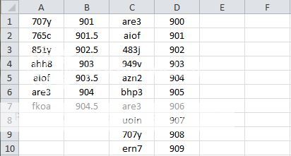
Example of the data:
A B C D E F
1 707y 901.0 are3 900
2 765c 901.5 aiof 901
3 851y 902.5 483j 902
4 ahh8 903.0 949v 903
5 aiof 903.5 azn2 904
6 are3 904.0 bhp3 905
7 fkoa 904.5 are3 906
8 Uoin 907
9 707y 908
10 Ern7 909
(Edit: sorry, the above looked like a true table when I typed it out)
The match formula in column E that I am using to initially match the cells in column A with anything in column C is: =IF(ISNA(MATCH(LEFT(A1,4)&"*",C:C,0)),NA(),A1) … (this includes matching the left 4 numbers with wildcards if a cell isn’t just 4 numerals long – sometimes there may be 5 or 6 digits) but now I need the formula to go one step further and if there is a potential match, the value of column B must also be greater than the value of column D in order to be returned in column E as a true match.
From the above data, I expect matches to result in E5 and E6 because they match and the value in column B is greater than in column D for the potential match. There would not be a “match” result in E1, however, because although the value in column A matches with something in column C, the associated value in column B (B1) is not greater than the associated value in column D (D9).
If it helps: This is in reference to a vehicle license plate study where we were stationed at two checkpoints collecting license plates. If a vehicle’s license plate was recorded at both checkpoints, it is a “match”, but in order to weed out duplicate plates, the only way they are a true match is if the timestamp at the second checkpoint is greater than the timestamp at the first checkpoint (this has to be - due travel time).
I also tried using =VLOOKUP(D1,$A:$B,2,0) in column E, after which I could then create another formula in column F to do a greater than comparison and then get my true matches, but I think VLOOKUP requires an exact match and the values won’t always be 4 numerals – sometimes “ahh8” will need to match “ahh87”. One final wrinkle is that there may be multiple duplicates in either column A or C that have allowable (greater than) timestamp values. But that may just complicate it further so I won’t worry about them.
If this is impossible in one forumula, doing multiple forumulas in more than one column is fine. Also, If I can provide more information I’ll be happy to.
I'm using Excel 2010.
Thank you
New user here - I’ve spent a lot of time searching for help but can’t find my exact situation so I’m posting this thread.
I’m trying to determine if a value in a cell from column A is matched in column C, but only under the condition that the associated column B is greater than column D.
I found a good matching formula from an answer to a question on this site, but I think I somehow need to add in an “AND” function to include the check of column B and column D.
Example of the data:
A B C D E F
1 707y 901.0 are3 900
2 765c 901.5 aiof 901
3 851y 902.5 483j 902
4 ahh8 903.0 949v 903
5 aiof 903.5 azn2 904
6 are3 904.0 bhp3 905
7 fkoa 904.5 are3 906
8 Uoin 907
9 707y 908
10 Ern7 909
(Edit: sorry, the above looked like a true table when I typed it out)
The match formula in column E that I am using to initially match the cells in column A with anything in column C is: =IF(ISNA(MATCH(LEFT(A1,4)&"*",C:C,0)),NA(),A1) … (this includes matching the left 4 numbers with wildcards if a cell isn’t just 4 numerals long – sometimes there may be 5 or 6 digits) but now I need the formula to go one step further and if there is a potential match, the value of column B must also be greater than the value of column D in order to be returned in column E as a true match.
From the above data, I expect matches to result in E5 and E6 because they match and the value in column B is greater than in column D for the potential match. There would not be a “match” result in E1, however, because although the value in column A matches with something in column C, the associated value in column B (B1) is not greater than the associated value in column D (D9).
If it helps: This is in reference to a vehicle license plate study where we were stationed at two checkpoints collecting license plates. If a vehicle’s license plate was recorded at both checkpoints, it is a “match”, but in order to weed out duplicate plates, the only way they are a true match is if the timestamp at the second checkpoint is greater than the timestamp at the first checkpoint (this has to be - due travel time).
I also tried using =VLOOKUP(D1,$A:$B,2,0) in column E, after which I could then create another formula in column F to do a greater than comparison and then get my true matches, but I think VLOOKUP requires an exact match and the values won’t always be 4 numerals – sometimes “ahh8” will need to match “ahh87”. One final wrinkle is that there may be multiple duplicates in either column A or C that have allowable (greater than) timestamp values. But that may just complicate it further so I won’t worry about them.
If this is impossible in one forumula, doing multiple forumulas in more than one column is fine. Also, If I can provide more information I’ll be happy to.
I'm using Excel 2010.
Thank you
Last edited: