MATCH function

[T1991]

I have two sheets:
Master sheet
Supporting sheet
I am trying to pull any names from column G in Master to column C in Supporting but only if the row meets the following requirements:
The values in columns H, I and J in Master match the cells A11, B10 and A4 in Supporting.
I only want it to pull the first instance of the name and then move onto the next one. I have copied this formula as an array into C11:C20 in Supporting:
=IFERROR(INDEX(Master!$G$3:$G$100, MATCH(0, COUNTIF($C$10:C10, Master!$G$3:$G$100) + IF((Master!$H$3:$H$100=$A11)*(Master!$I$3:$I$100=B$10)*(Master!$J$3:$J$100=$A$4), 1, 0), 0)), "")

Additionally, I want to take a similar approach for column F in Supporting, where the match requirement will change from:
Master!$I$3:$I$100=B$10 to Master!$I$3:$I$100=E$10

However it just keeps pulling the same names from column C.

Any advice would be more than welcome. I have been on this for days

 

[Fluff]

What version of Excel are you using?

I suggest that you update your Account details (or click your user name at the top right of the forum) so helpers always know what Excel version(s) & platform(s) you are using as the best solution often varies by version. (Don’t forget to scroll down & ‘Save’)

 

[T1991]

What version of Excel are you using?

I suggest that you update your Account details (or click your user name at the top right of the forum) so helpers always know what Excel version(s) & platform(s) you are using as the best solution often varies by version. (Don’t forget to scroll down & ‘Save’)

Apologies, it's 2016.

 

[Fluff]

Thanks for that.
How about in C11 dragged down

=IFERROR(INDEX(Master!G:G,AGGREGATE(15,6,ROW(Master!$G$3:$G$100)/(Master!$H$3:$H$100=$A$11)/(Master!$I$3:$I$100=$B$10)/(Master!$J$3:$J$100=$A$4)/(ISNA(MATCH(Master!$G$3:$G$100,C$10:C10,0))),1)),"")

 

[T1991]

Thanks for that.
How about in C11 dragged down

=IFERROR(INDEX(Master!G:G,AGGREGATE(15,6,ROW(Master!$G$3:$G$100)/(Master!$H$3:$H$100=$A$11)/(Master!$I$3:$I$100=$B$10)/(Master!$J$3:$J$100=$A$4)/(ISNA(MATCH(Master!$G$3:$G$100,C$10:C10,0))),1)),"")

Thanks for responding.

So it pulls the first name from column G in Master, but not the next name. Every new entry in Master sits above the last one. I don't know if that's relevant?

 

[T1991]

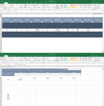
I have attached a picture of the layout...

 

[Fluff]

From what I can see it's pulling the last entry, not the 1st.
Check that the data in cols H, I & J are an exact match to the criteria.

 

[T1991]

From what I can see it's pulling the last entry, not the 1st.
Check that the data in cols H, I & J are an exact match to the criteria.

Sorry, so the oldest entry, i.e. the first is the one on the bottom - Joe Bloggs. Newer entries automatically go on top via a User Form / VBA.

I have checked all of the columns and they do indeed match. I used a formula to double check the individual columns too.

Having such a nightmare with this sheet

 

[Fluff]

Sorry, so the oldest entry, i.e. the first is the one on the bottom

That doesn't change the fact that it is not pulling the 1st entry (ie the row 7)

Can you post some sample data.
MrExcel has a tool called “XL2BB” that lets you post samples of your data that will allow us to copy/paste it to our Excel spreadsheets, so we can work with the same copy of data that you are. Instructions on using this tool can be found here: XL2BB Add-in

Note that there is also a "Test Here” forum on this board. This is a place where you can test using this tool (or any other posting techniques that you want to test) before trying to use those tools in your actual posts.

 

[T1991]

This is the Master sheet...

Template.xlsm
	A	B	C	D	E	F	G	H	I	J	K
1	< Input data
2	DEPARTMENT	REQUEST ID	POSITION NUMBER	SOURCE	BACKFILL / ADDITIONAL	APPROVED FROM	FORMER ROLE OCCUPANT	OU SHORT-CODE	CONTRACT TYPE	END DATE (MM/YY)	MANAGER
3	... | P
4	... | PC
5	... | PL
6	... | PS
7	… | PS	E	F	G	Backfill	H	John Doe	PS	Exec	01/24
8	... | PS	A	B	C	Backfill	D	Joe Bloggs	PS	Exec	01/24
9	... | PP
10	... | PM
11	... | PI
12	... | PV
Master

This is the Supporting sheet...

Template.xlsm
	A	B	C	D	E	F	G	H	I	J	K	L	M	N	O	P
1					Budget:		47	Plan:		47
2	Memo:
3
4	01/24										Non-payroll:			…
5	AOR
6	Totals	Exec			Staff			Indirect			Direct			External
7
8
9
10		Exec			Staff			Indirect			Direct			External
11	PS		Joe Bloggs
12
13
14
15
16
17
18
19
20
21	PSK
22	PSS
23	PSX
24	QUERY
Supporting

Cell Formulas
Range	Formula
C11,C21:C24	C11	=IFERROR(INDEX(Master!$G$3:$G$101,MATCH(1,(Master!$H$3:$H$101=$A11)*(Master!$I$3:$I$101=B$10)*(Master!$J$3:$J$101=$A$4),0)),"")
Press CTRL+SHIFT+ENTER to enter array formulas.