Consolidate Data, Combine Text, and Calculate Age

[VtQuest]

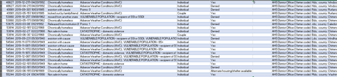
I am working with a spreadsheet regarding housing for homeless people. The people are represented by ID numbers. There are many duplicates. I want to sum SOME of the values associated with the IDs while also combining text notes. The values I wish to sum are Number of Nights. I wish to combine the text in the Causes column and in the Housing Authorized column (separately). I’d also like to calculate age from birthdates, and number of calls based on call date. (Call date is not listed in the first example.)

I have familiarity with Excel in its simple form, not at this level. (I’m sure, to some people, this is pretty simple, but not to me - yet.) So, I’m not familiar with many formula terms or query tools. Please respond with this in mind.

The first image is a sample of the data, with identifying information obscured. The second image is of the desired result.

Thank you for your help.

 

[VtQuest]

Hi Paul,

I must be doing something wrong. I pasted my spreadsheet into the Data tab, and pasted the list of unduplicated client IDs into the first column of Report 1. It processed (if that's the word?) about 17 rows, but the middle cells of the remaining cells were blank. Prior to pasting the IDs, I had copied the formulas to over 2500 rows, based on how many IDs I was going to input. I've removed the IDs -- they're in a tab at the beginning of the spreadsheet. Can you please explain what I could be doing wrong?

I'm not sure how to share the spreadsheet - I added it to dropbox and tried to share, but that required an email.

Login - Dropbox

Login to Dropbox. Bring your photos, docs, and videos anywhere and keep your files safe.

www.dropbox.com

Please also let me know how to post a dropbox document to Mr. Excel.

Thanks very much,
Beth

 

[Taul]

Hi,
When you copy the formulas down on report 1, there is no need to include column "B" (the yellow cells), they can remain blank until you are ready to paste the unique list of ID numbers.
You only mentioned there was a problem with Report 1, as all reports read from the Data page, are the other reports working as expected?

When you say "Middle cells" is that columns E, F, G & H, if so, they are all array formulas. If you clicked in the formula bar during you copy paste process, they may no longer be array formulas. The array formula should have curly brackets at the start and finish of the formula, could you check if they are still there. Also, are the cells displaying #VALUE!

You may notice that reports 3 & 5 use a formula to generate the unique ID list, It may be better to use the same formula on report 1
Also, you mentioned you had made some changes to the raw data, Just in case the layout has changed, could you post a screenshot of your raw data. Please "doctor" sensitive things but I'm interested in seeing the current layout and the way the data looks. If possible, could you ensure there data is representative of all the different types of categories. I'm guessing about 10 to 20 rows of data should do it.

If you want to pursue the dropbox option, you will first have to create an account with dropbox before you can upload a file. When the file is uploaded, you click on the Share with Dropbox and click on copy the link. The link copy is held in your clipboard so you can then paste the link into the forum page.

 

[VtQuest]

Hi Paul,

I'm sorry I've gotten so screwed up in how I'm doing this. I'm usually a fast learner with tech stuff, but not this time.

This should be a link to the dropbox file: Forum Q - Rev3 Try2.xlsm

Here are my responses to your notes:

When you copy the formulas down on report 1, there is no need to include column "B" (the yellow cells), they can remain blank until you are ready to paste the unique list of ID numbers. I'll remember that for next time.
You only mentioned there was a problem with Report 1, as all reports read from the Data page, are the other reports working as expected?
Report 2 appears to have worked; Report 3 only goes to row 24; 4 and 5 have #VALUE showing

When you say "Middle cells" is that columns E, F, G & H, if so, they are all array formulas. If you clicked in the formula bar during you copy paste process, they may no longer be array formulas. The array formula should have curly brackets at the start and finish of the formula, could you check if they are still there. Also, are the cells displaying #VALUE! The copied cells do have the curly brackets at start and finish of the formula.

You may notice that reports 3 & 5 use a formula to generate the unique ID list, It may be better to use the same formula on report 1 Would I put that formula in column B in Report 1?
Also, you mentioned you had made some changes to the raw data, Just in case the layout has changed, could you post a screenshot of your raw data. Please "doctor" sensitive things but I'm interested in seeing the current layout and the way the data looks. If possible, could you ensure there data is representative of all the different types of categories. I'm guessing about 10 to 20 rows of data should do it. I think the raw data I changed was the Points section; I replaced the entry with Points: #. So, what you'll see below is the result of that.

Thank you,
Beth

 

[Taul]

Hi,
I think I have spotted the source or the error, actually there are several problems.
There are two columns on the Data page (columns B & C) that contain dates. These are not real dates, they are actually TEXT that look like dates. This causes the formula to have a hissy fit, or more accurately causes a #VALUE! error.

Column "C" is the date of birth. The age formula can handle the text ok and is showing the age of the person where the month column is 12 or less. This is because the sheet I produced has been created in the UK with English (UK) location, and you will need English (US) location with "US" date formats.
e.g. cell C7 is showing 01/03/1971 and the age calculation is reading this as 1st March 1971. In fact it is January 3rd 1971, so the age calculation is producing an answer in some of the cells but it is the wrong answer. Other cells showing a #VALUE! error are because the month that is being read is greater than 12.
There are several ways to convert text dates to real dates and I have tried a few with no result, like multiplying by 1 to force a calculation and hence the conversion, using text to columns etc but so far no luck.
Column "B" is the date of registration, where we have the same location issue but in addition the date has additional text, typically 2020-02-08T00:00;00-05:00

I assume this data is downloaded from a database, is this correct?
If so, you could have a word with the person that manages the database and ask they modify the export routine to format the dates as real dates and not as text. I think this would save a lot of heartache.
Meanwhile, I will need more time to find an appropriate solution, its late here so I will look at it again tomorrow.

cheers
Paul.

 

[VtQuest]

Hi Paul,

I see what you mean. I am off today but will return to this tomorrow and contact the database company. I have little faith that they will change the date information for me. But changing the date information into text makes sense!

Thank you,
Beth

 

[Taul]

I temporarily changed my computer regional settings from UK to USA, so hopefully I can see what you see. I immediately noticed all the age calculations corrected.
Ok, there are a few errors but that is because some of the original dates in column B on the Data page are wrong.
That is to say the date is missing or written incorrectly like:-
00/88/0275
00/85/0267
01/09/1987;07/24/1970 (yes, it is actually one text string in a cell)
12/31/8198
12/51/1981

I think you will have to use the Autofilter on column C and manually correct the dates.

To convert the dates on the Data page in column B (Registered Dates)
Select the whole range. The easy way is to click on cell B2 then use the keyboard shortcut Ctrl+shift+down arrow to select the whole column.
The on the “Data” ribbon, click on “Text to Columns”, click “Next” and “Next” again, then click on the button for “Date”. In the window to the right of that select “DMY”.
Then click “Finish”
The TEXT dates will have been converted to real dates. You can now “Format” the dates as you wish to see them (its optional). To format the dates go to the “Home” ribbon, on the far right click on “Format”, in the drop down select “Format Cells” and choose the format you want to use.

I have already done the exercise of converting the TEXT date to real dates, so you should be able to use the new file called “Rev3 Try3 form Paul”. But it would be worth doing it yourself, so you are familiar with the process.

I’m not sure how often you will need to run this report, is it a one-off exercise or will it need to be run weekly, monthly or just at the end of the year? It only matters because if it is a regular thing, then we should automate it as much as possible.

Cheers
Paul.

Forum Q - Rev3 Try3 from Paul.xlsm

Shared with Dropbox

www.dropbox.com

 

[VtQuest]

Hi Paul,

Thank you for your response. I've had to spend the whole day working on updating our information about winter homeless shelters, and Thanksgiving programs for people in need, plus updating our website. Sorry I haven't been able to get to this today, but will on Monday.

Ciao,
Beth

 

[Taul]

Hi Beth,
I have taken the liberty of changing a few things, I hope you don't mind. There is a list of changes on a separate page tab on the Rev 4 file
cheers
Paul

Forum Q - Rev4.xlsm

Shared with Dropbox

www.dropbox.com

 

[VtQuest]

Hi Paul,
Thanks soch for all of the changes you've made. Nice graph in Report4! Nearly everything seems to be complete. I just have a few questions about how to proceed.

You refer to column Y in the yellow "Data" tab, but I'm not sure what you're referring to -- it just seemed blank - no formulas or data.

Would it be ok if I wanted to sort columns differently, say, in Report 1 to see the highest number of motel stays?

Would it help if I manually corrected the locations you listed in the Unique ID tab?

That is odd about the misspelled word (I know, American English has its own word for misspelt) - I will let the database manager know (or perhaps it's how the descriptor is set up in a dropdown menu for our I&R specialists). I&R Information and Referral.

I think most of the reports are useful; some perhaps beyond my initial impressions - to be discovered. I'll be forwarding this to my boss to see if she has any questions.
In Report 3, using the Autofilter, should I try to come up with likely substitutes? Also in that report, it looks like you already pasted in the unique IDs. Correct?

In Report 6, I would like to play around with this kind of report, but see that it ends at row 16. How do I get it to continue through all of the IDs?

Thank you so much for all of the time and effort you've put into these reports -- and attempts to explain things to me. I'm really truly grateful!

Beth

 

[Taul]

Hi Beth,
Just to address your questions:-

“You refer to column Y in the yellow "Data" tab, but I'm not sure what you're referring to -- it just seemed blank - no formulas or data.”
Column “Y” in the yellow data page is wrong (my bad), I should have said column “B”, it was late and I was getting glazed eyes. Basically I used the Text to Columns method to convert the text dates to real dates in the raw data. This was done by you initially but I did it again for columns B & C to make sure.

“Would it be ok if I wanted to sort columns differently, say, in Report 1 to see the highest number of motel stays?”
For the highest number of motel stays (# of Nights) it would best not to change the order of the raw data, unless you want earliest or latest date recordings of a unique ID number.
For example, an ID number may record a person as a single person. The next occurrence of that same ID number may record that same person as a couple (due to the circumstances of the person when interviewed or an error in recording) so your reports may give different results depending how the data is sorted. For consistency, it is best to leave the raw data alone.

The best way to get the highest number of nights is to either generate a new report or go to Report 3 and use the AutoFilter on column “AF”, click on the values say 29 to 11 to generate a filtered list of the highest number of nights or all of them if you prefer. You can then copy and Paste as Values to another page.
You can use “Paste Special” to:-
Paste column widths
Paste as Values
Paste formats

“Would it help if I manually corrected the locations you listed in the Unique ID tab?”
Yes, by all means change the raw data in this instance. You can use “Find and Replace” to do it.
You will also need to correct the spelling in the following locations:-
Report 2, cell B23
Report 3, cell R5
Report 4, cell B22

Good point about misspelt vs misspelled. It depends which side of the pond we are on. Someone famous once said “We are divided by a common language”.
Best way to avoid the location name problem is to have a drop down menu available to the people collecting the data.
As soon as you let a human loose to type whatever they want into a text box, then trying to collate the data for a report will be problematic.

“In Report 3, using the Autofilter, should I try to come up with likely substitutes? Also in that report, it looks like you already pasted in the unique IDs. Correct?”
Yes I already pasted the unique ID numbers.
Using the AutoFilter to find the incorrectly entered dates is ok. When you have found them I’m not sure what to do about them. Perhaps use Report 3, AutoFilter column “AF” and select the wrong dates and the unknown dates and then copy the filtered list to a new location, same Paste Special method as mentioned above. At least you will be able to report something about the data.

“In Report 6, I would like to play around with this kind of report, but see that it ends at row 16. How do I get it to continue through all of the IDs?”
Report 6 is a Pivot Table.
As a general rule, if you have a large amount of data and you need to extract reports, then a pivot table is the best way to go.
Having said that, I am ashamed to admit that I don’t use them much, which is why I suggested you take a look at some YouTube vids to see their versatility.
When I put the pivot table onto the page, I only had limited rows of sample data. You now need to extend the range.
Click once in the pivot table and the PivotTable fields will appear on the right hand side of the page. At the same time you will notice two additional tabs in the ribbon at the top of the page “Analyze & Design”.
Click on Analyze
Click on “Change PivotTable Data Source”
Change the range from Data!$A$1:$K$34 to Data!$A$1:$K$4799
Click “OK”
This will produce a very long list of ID numbers, so you will need to play around with the Fields.

I hope this is of some assistance.
Cheers
Paul.