Count multiple conditions

[yipppppppy]

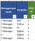
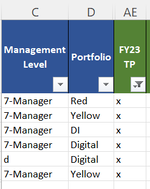
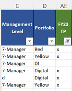
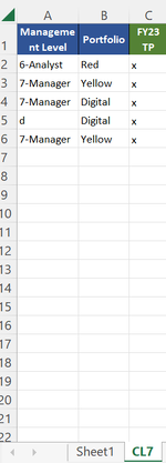
Hi all, the following formula is returning 4 rows. The answer should be 1. I am trying to get the formula to only count a row where it meets all 3 conditions below
1) FY23 TP has an x AND
2) Portfolio is either DI, DD or Digital AND
3) Management Level is 7-Manager OR 6-Analyst

=SUMPRODUCT(--IF(OR('CL7'!D:D="DD",'CL7'!D:D="DI",'CL7'!D:D="Digital"),FILTER(('CL7'!A1:AO1="FY23 TP")*('CL7'!A:AO="x"),'CL7'!C:C="7-Manager")))

IMPORTANT: Can you please update the formula so it is more tighter just incase i need to shuffle these columns around? E.g. if i want to move Management Level to Column Z or any other Column etc. Same with the other two columns Portfolio and FY23 TP

 

[Peter_SSs]

I would strongly recommend against using whole column references in a SUMPRODUCT formula. below I have used down to row 1,000. Just make sure that is a big enough number to cover any data you might have,

yipppppppy.xlsm
	C	D																											AE
1	Management Level	Portfolio																											FY23 TP
2	7-Manager																												x
3	6-Analyst																												x
4	7-Manager	DD																											x
5																													x
6	7-Manager	DD
7																													x
8																													x
9	7-Manager	DI																											x
10
11	d	Digital																											x
12																													x
13
CL7

Try this formula for the count

yipppppppy.xlsm
	A
1	2
Sheet2

Cell Formulas
Range	Formula
A1	A1	=LET(h,'CL7'!A1:AO1,r,'CL7'!A2:AE1000,m,INDEX(r,0,MATCH("Management Level",h,0)),p,INDEX(r,0,MATCH("Portfolio",h,0)),fy,INDEX(r,0,MATCH("FY23 TP",h,0)),IFNA(ROWS(FILTER(m,(m="7-Manager")*((p="DD")+(p="DI")+(p="Digital"))*(fy="x"),NA())),0))

 

[yipppppppy]

Thanks. Your formula returned zero as per second screenshot below. Please note: First screenshot is in a seperate tab (Tab name is CL7) to the second screenshot (Tab name is Sheet 1)

 

[yipppppppy]

Also i think your formula doesnt factor in any rows the third condition if a row met the first two points below and the third point is an 6-Analyst.

1) FY23 TP has an x AND
2) Portfolio is either DI, DD or Digital AND
3) Management Level is 7-Manager OR 6-Analyst

The answer should be 1, not 0 based on the table i pasted just above.

 

[Peter_SSs]

You can see that the formula worked for me. That indicates likely something different about your data but we can't tell much from an image.
Can you post those two small sheet sections again, but with XL2BB* so we can copy to test with your data, not ours?

* .. or as I mentioned in my conversation message to you about another thread.

3) Management Level is 7-Manager OR 6-Analyst

Yes, I missed that OR and will address that when the other problem is resolved.

 

[yipppppppy]

Hi,

Unfortunately it is not allowing me to add it as it is being blocked by my organisation (its a work computer).

I have copied the full screenshot including the tab for each if it helps?

 

[Peter_SSs]

Images still don't help.
Options:

• Check for trailing (or leading) space characters with any of the data.
• Start a new test workbook and manually type in a few values in those columns and test that. Or you can copy my test data with this:
  
  
• Share a dummy workbook as I suggested in my conversation message.

With the missed condition ..

yipppppppy.xlsm
	C	D																											AE
1	Management Level	Portfolio																											FY23 TP
2	7-Manager																												x
3	6-Analyst																												x
4	7-Manager	DD																											x
5																													x
6	7-Manager	DD
7	6-Analyst	Digital																											x
8																													x
9	7-Manager	DI																											x
10
11	d	Digital																											x
12																													x
CL7

yipppppppy.xlsm
	A
1	3
Sheet 1

Cell Formulas
Range	Formula
A1	A1	=LET(h,'CL7'!A1:AO1,r,'CL7'!A2:AO1000,m,INDEX(r,0,MATCH("Management Level",h,0)),p,INDEX(r,0,MATCH("Portfolio",h,0)),fy,INDEX(r,0,MATCH("FY23 TP",h,0)),IFNA(ROWS(FILTER(m,((m="7-Manager")+(m="6-Analyst"))*((p="DD")+(p="DI")+(p="Digital"))*(fy="x"),NA())),0))

 

[Peter_SSs]

@yipppppppy
I think that you may have looked at an incorrect version of my last post. I had an error in the Sheet 1 formula in that I was referencing a different number of columns for the main data compared to the headings. I have since edited the mini sheet with the formula to correct that. Both headings and data now look at columns A:AO.

 

[yipppppppy]

Ok no worries. I have literally deleted the CL7 tab with all the data there. Created a completely new tab titled CL7 and entered only the following to the new CL7 tab. Copied the raw data below and the corresponding screenshot further below.

Once i copy this formula to the Sheet1 tab i still get zero.

=LET(h,'CL7'!A1:AN1,r,'CL7'!A2:AD1000,m,INDEX(r,0,MATCH("Management Level",h,0)),p,INDEX(r,0,MATCH("Portfolio",h,0)),fy,INDEX(r,0,MATCH("FY23 TP",h,0)),IFNA(ROWS(FILTER(m,((m="7-Manager")+(m="6-Analyst"))*((p="DD")+(p="DI")+(p="Digital"))*(fy="x"),NA())),0))

Management Level	Portfolio	FY23 TP
6-Analyst	Red	x
7-Manager	Yellow	x
7-Manager	Digital	x
d	Digital	x
7-Manager	Yellow	x

 

[Peter_SSs]

Once i copy this formula to the Sheet1 tab i still get zero.

Gives 1 for me. Can you share the workbook with that latest small data?