Hi,
I'm sure that it's very easy question and there is an easy way to do that, but I don't know why now it's not in my mind.
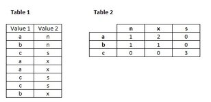
Look the image attached. For each cell, I would use an excel formula that allows to get the values on Table2 starting from Table1. I don't want to use a pivot table.
Thanks
I'm sure that it's very easy question and there is an easy way to do that, but I don't know why now it's not in my mind.
Look the image attached. For each cell, I would use an excel formula that allows to get the values on Table2 starting from Table1. I don't want to use a pivot table.
Thanks
Attachments
Last edited:
")


