Countif based on dates within a column

[Sifuevs]

Hi,
I am relatively new to Excel and I am looking for help with a formula.
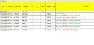
So all my data is stored in the data tab (see attached image). I have another tab that will calculate and display results, the summary tab (see attached image).
So I want to the formula to do the following:
Column A in the data tab contains date. If any date within the column contains the month of Feb for instance then COUNTA(Data!C2:C4624.
I did try some formula but keep getting a spill error (as I am a novice I am not sure what I am doing wrong, sorry).

Thanks for help

 

[awoohaw]

You're creating a spilled array, for each cell in the range A2:A4624 excel wants to place a value in the 4623 cells below the cell where you see the SPILL# message.

There are a number of ways to get around this, but some solutions may not work in your excel version. Can you please update your profile so your excel version shows up on your profile button (see how mine says 365?).

But, one way that should work for most versions of excel is:

=SUMPRODUCT((MONTH(Data!A2:A4624)=2)*(Data!C2:C4624<>""))

 

[Alex Blakenburg]

Please go into your Mr Excel Account Profile and update what version of Excel you are using. (Oops duplicated the above here )
If you are using pre MS365 / O2021 the Awoohaw's method would be the way to go.

Since you are getting #SPILL I suspect you have MS365, in which case something like this might work for you.

=COUNTA(FILTER(Data!$C$2:$C$4624,MONTH(Data!$A$2:$A$4624)=2,""))

 

[Sifuevs]

You're creating a spilled array, for each cell in the range A2:A4624 excel wants to place a value in the 4623 cells below the cell where you see the SPILL# message.

There are a number of ways to get around this, but some solutions may not work in your excel version. Can you please update your profile so your excel version shows up on your profile button (see how mine says 365?).

But, one way that should work for most versions of excel is:

=SUMPRODUCT((MONTH(Data!A2:A4624)=2)*(Data!C2:C4624<>""))[/
[/QUOTE]

You're creating a spilled array, for each cell in the range A2:A4624 excel wants to place a value in the 4623 cells below the cell where you see the SPILL# message.

There are a number of ways to get around this, but some solutions may not work in your excel version. Can you please update your profile so your excel version shows up on your profile button (see how mine says 365?).

But, one way that should work for most versions of excel is:

=SUMPRODUCT((MONTH(Data!A2:A4624)=2)*(Data!C2:C4624<>""))

Thanks for your reply. I have now updated my profile and yes I am using 365.
The formula worked but it discards any dates that are the same. I need the count to include dates that are the same. So I can get a total line qty of all dates falling with the month of Feb.
Thanks again. Much appreciated

 

[Sifuevs]

Please go into your Mr Excel Account Profile and update what version of Excel you are using. (Oops duplicated the above here )
If you are using pre MS365 / O2021 the Awoohaw's method would be the way to go.

Since you are getting #SPILL I suspect you have MS365, in which case something like this might work for you.

=COUNTA(FILTER(Data!$C$2:$C$4624,MONTH(Data!$A$2:$A$4624)=2,""))[/CODE
[/QUOTE]
Thanks for your reply.
With this formula I get a notification box "This function is not valid"?

 

[awoohaw]

not sure what you mean? the Month(cellref)=2 function will get only February records, and the cellref<>"" will get the non blanks.
Please post some examples of what you think should have been included? The xl2bb add in (link below) is very helpful with that.

 

[Sifuevs]

not sure what you mean? the Month(cellref)=2 function will get only February records, and the cellref<>"" will get the non blanks.
Please post some examples of what you think should have been included? The xl2bb add in (link below) is very helpful with that.

Sorry, my mistake. The formula works perfect. Thank you
I also have other formula that needs to do the same, look to see if column A values fall in the month of Feb and if so then do this =COUNTIFS(Data!$G$3:$G$4625,"REPLEN",Data!$I$3:$I$4625,"A")
Is this possible or too much?
Again much appreciate your help.
This forum is a god send and I value you guys so much.

 

[awoohaw]

i'm guessing you want to count the number of "REPLEN" in column G, that occur when Column A has a month of February.

=SUMPRODUCT((MONTH(Data!A2:A4624)=2)*(Data!G2:G4624="REPLEN"))

I don't know what you're checking in column I.

 

[Sifuevs]

not sure what you mean? the Month(cellref)=2 function will get only February records, and the cellref<>"" will get the non blanks.
Please post some examples of what you think should have been included? The xl2bb add in (link below) is very helpful with that.

Sorry, my mistake. The formula works perfect. Thank you
I also have other formula that needs to do the same, look to see if column A values fall in the month of Feb and if so then do this =COUNTIFS(Data!$G$3:$G$4625,"REPLEN",Data!$I$3:$I$4625,"A")
Is this possible or too much?
Again much appreciate your help.
This forum is a god send and I value you guys so much.

i'm guessing you want to count the number of "REPLEN" in column G, that occur when Column A has a month of February.

=SUMPRODUCT((MONTH(Data!A2:A4624)=2)*(Data!G2:G4624="REPLEN"))

I don't know what you're checking in column I.

So sorry.
So if the dates in data range A2:A4624 = the month of Feb and if data in G2:G4624="Replen" and if code in data range I3:I4624 = "A" then count the qty of lines.
Hope this makes more sense.
Again thanks for your help.

 

[Alex Blakenburg]

Just follow the pattern that awoohaw is using:

=SUMPRODUCT( (MONTH(Data!A2:A4624)=2) * (Data!G2:G4624="REPLEN") * (Data!I2:I4624="A") )