Countif with multiple criteria

[vladi305]

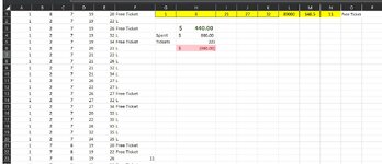
this worksheet checks that values on the range from A:E all the way down to match the one from G:K on the first row

I tried using COUNTIFS, MATCH with SUM, SUMPRODUCT and the best I could do was hardcoding the array. It will be productive to change this to check the values from G to K dinamically and not hardcode as it is
Any ideas to improve this formula?

=IF(SUM(COUNTIF(A1:E1,{"8","19","26","27","34"}))=5,$L$1,
IF(SUM(COUNTIF(A1:E1,{"8","19","26","27","34"}))=4,$M$1,
IF(SUM(COUNTIF(A1:E1,{"8","19","26","27","34"}))=3,$N$1,
IF(SUM(COUNTIF(A1:E1,{"8","19","26","27","34"}))=2,$O$1,
IF(SUM(COUNTIF(A1:E1,{"8","19","26","27","34"}))<2,"L","F")))))

 

[etaf]

the "8" is looking for text , not a number
perhaps a sumproduct
=SUMPRODUCT(--(A1:E1=G1:K1))
within the IF()

BUT you say you tried that already - or at least sumproduct

Note: Images are difficult to see , and also requires that I input all the data myself, which means I may make an error, which is very time consuming, and from my point of view less likely to get a response, if a complicated spreadsheet. Plus we cannot see any of the formulas used.

Therefore -

A SMALL sample spreadsheet, around 10-20 rows, would help a lot here, with all sensitive data removed, and expected results mocked up and manually entered, with a few notes of explanation.

MrExcel has a tool called “XL2BB” that lets you post samples of your data and will allow us to copy/paste your sample data into our Excel spreadsheets, saving a lot of time.

XL2BB - Excel Range to BBCode

Excel 'mini-sheet' in messages - XL2BB Although experts prefer to read your description and question instead of working in your actual file to solve your problem, there are times that it is difficult to explain an issue without providing actual...

www.mrexcel.com

You can also test to see if it works ok, in the "Test Here" forum.

Test Here

Use this forum to test your signature, learn bbcode, smilies, XL2BB, etc. Threads in this forum are automatically deleted after no replies for seven (7) days

www.mrexcel.com

OR if you cannot get XL2BB to work, or have restrictions on your PC , then put the sample spreadsheet onto a share
I only tend to goto OneDrive, Dropbox or google docs , as I'm never certain of other random share sites and possible virus.
Please make sure you have a representative data sample and also that the data has been desensitised, remember this site is open to anyone with internet access to see - so any sensitive / personal data should be removed

 

[Skyybot]

This formula in cell F1 then copy and paste formula for the rest of the rows in column F.

=IF(AND(A1=$G$1,B1=$H$1,C1=$I$1,D1=$J$1,E1=$K$1),"F","L")

 

[Skyybot]

This formula in cell F1 then copy and paste formula for the rest of the rows in column F.

=IF(AND(A1=$G$1,B1=$H$1,C1=$I$1,D1=$J$1,E1=$K$1),"F","L")

I may have reversed the "F" and the "L" for your application.

 

[kvsrinivasamurthy]

Try this ARRAY formula.

=IF(SUM(COUNTIF(A1:E1,{"8","19","26","27","34"}))={5,4,3,2,1},$L$1:$O$1,IF(SUM(COUNTIF(A1:E1,{"8","19","26","27","34"}))<2,"L","F"))

To enter ARRAY formula
Copy and paste the formula in cell
Press F2
Press Ctrl+Shift+Enter together
Excel covers the formula with {}.

 

[hajiali]

not sure if this is what you're looking for. I would arrange your Excel like the one below.

Mrexcel.xlsm
	A	B	C	D	E	F	G	H	I	J	K	L	M	N	O	P
1	1	8	7	19	20	Free Ticket	1	8	21	27	32	1	2	3	4	5
2	1	2	7	19	22	L						L	Free Ticket	11	148.5	89000
3	1	2	7	19	26	L
4	1	2	7	19	32	Free Ticket
5	1	2	7	19	34	L
6	1	2	7	20	21	Free Ticket
7	1	2	7	21	22	Free Ticket
8	1	2	7	21	26	Free Ticket
9	1	2	7	21	32	11
10	1	2	7	21	34	Free Ticket
Sheet1

Cell Formulas
Range	Formula
F1:F10	F1	=IFERROR(INDEX($L$1:$P$2,2,MATCH(SUM(COUNTIF(A1:E1,$G$1:$K$1)),$L$1:$P$1,0)),"F")

 

[kvsrinivasamurthy]

Formula in Post#5 may not work in many conditions.
Assuming that A1:E1 are numbers not strings.
Try
=IFERROR(INDEX($L$1:$O$1,MATCH(SUM(COUNTIF(A1:E1,{8,19,26,27,34})),{5,4,3,2},0)),IF(SUM(COUNTIF(A1:E1,{8,19,26,27,34}))<2,"L","F"))

 

[vladi305]

Ty guys, I'll try some of the modified formulas here, the one I have works fine but it's hardcoded and numbers need to be inputed every time on a daily basis

 

[vladi305]

not sure if this is what you're looking for. I would arrange your Excel like the one below.

Mrexcel.xlsm
	A	B	C	D	E	F	G	H	I	J	K	L	M	N	O	P
1	1	8	7	19	20	Free Ticket	1	8	21	27	32	1	2	3	4	5
2	1	2	7	19	22	L						L	Free Ticket	11	148.5	89000
3	1	2	7	19	26	L
4	1	2	7	19	32	Free Ticket
5	1	2	7	19	34	L
6	1	2	7	20	21	Free Ticket
7	1	2	7	21	22	Free Ticket
8	1	2	7	21	26	Free Ticket
9	1	2	7	21	32	11
10	1	2	7	21	34	Free Ticket
Sheet1

Cell Formulas
Range	Formula
F1:F10	F1	=IFERROR(INDEX($L$1:$P$2,2,MATCH(SUM(COUNTIF(A1:E1,$G$1:$K$1)),$L$1:$P$1,0)),"F")

I'll use this method. I tried 4 and it didn't work and #5 is using hardcode numbers on the array so hajiali method was the best choice for my application. Again, thank you guys!

 

[vladi305]

the "8" is looking for text , not a number
perhaps a sumproduct
=SUMPRODUCT(--(A1:E1=G1:K1))
within the IF()

BUT you say you tried that already - or at least sumproduct

Note: Images are difficult to see , and also requires that I input all the data myself, which means I may make an error, which is very time consuming, and from my point of view less likely to get a response, if a complicated spreadsheet. Plus we cannot see any of the formulas used.

Therefore -

A SMALL sample spreadsheet, around 10-20 rows, would help a lot here, with all sensitive data removed, and expected results mocked up and manually entered, with a few notes of explanation.

MrExcel has a tool called “XL2BB” that lets you post samples of your data and will allow us to copy/paste your sample data into our Excel spreadsheets, saving a lot of time.

XL2BB - Excel Range to BBCode

Excel 'mini-sheet' in messages - XL2BB Although experts prefer to read your description and question instead of working in your actual file to solve your problem, there are times that it is difficult to explain an issue without providing actual...

www.mrexcel.com

You can also test to see if it works ok, in the "Test Here" forum.

Test Here

Use this forum to test your signature, learn bbcode, smilies, XL2BB, etc. Threads in this forum are automatically deleted after no replies for seven (7) days

www.mrexcel.com

OR if you cannot get XL2BB to work, or have restrictions on your PC , then put the sample spreadsheet onto a share
I only tend to goto OneDrive, Dropbox or google docs , as I'm never certain of other random share sites and possible virus.
Please make sure you have a representative data sample and also that the data has been desensitised, remember this site is open to anyone with internet access to see - so any sensitive / personal data should be removed

This formula worked fine as well, sorry I didn't try it before, I was looking at getting the complete formula and not just the counting