gtd526
Well-known Member
- Joined
- Jul 30, 2013
- Messages
- 657
- Office Version
- 2019
- Platform
- Windows
Hello,
Just wondering why its not counting correctly.
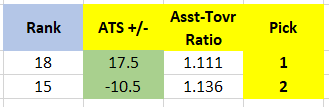
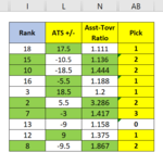
I, L, N = Values to Count according to CountIf in AB
AB = Countif
Just wondering why its not counting correctly.
I, L, N = Values to Count according to CountIf in AB
AB = Countif
| Cell Formulas | ||
|---|---|---|
| Range | Formula | |
| I5:I6 | I5 | =VLOOKUP($A5,TeamRankings!$DD:$DE,2,0) |
| L5:L6 | L5 | =IFERROR(VLOOKUP(A5,TeamRankings!$CX$3:$DC$33,6,0),"") |
| N5 | N5 | =IFERROR(VLOOKUP(A5,TeamRankings!AT3:AW32,4,0),"") |
| AB5 | AB5 | =COUNTIF(I5,"<"&I6)+COUNTIF(L5,">"&L6)+COUNTIF(N5,">"&N6) |
| N6 | N6 | =IFERROR(VLOOKUP(A6,TeamRankings!AT3:AW32,4,0),"") |
| AB6 | AB6 | =COUNTIF(I6,"<"&I5)++COUNTIF(L6,">"&L5)+COUNTIF(N6,">"&N5) |