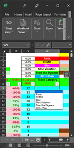
The attached picture shows column W with W7:W7 containing a list and color formatting. The table column below (Trades[Trade Category]) uses the list above for a drop down and I have Conditional formatting to match the colors. The percentages to the left are meant to be the percent of each category being displayed. I have the formula blow which works so long as no filter is applied to the table. The formulas dont give an error but they give unpredictable results when the table is filtered. I need to tweak the formula so that it works when the table is filtered.
=SUMPRODUCT((Trades[Trade Category]=W2)*(SUBTOTAL(103,OFFSET(W2,ROW(Trades[Trade Category])-MIN(ROW(Trades[Trade Category])),0))))/SUBTOTAL(103,Trades[Trade Date])
Trades[TradeDate] is present in every record.
=SUMPRODUCT((Trades[Trade Category]=W2)*(SUBTOTAL(103,OFFSET(W2,ROW(Trades[Trade Category])-MIN(ROW(Trades[Trade Category])),0))))/SUBTOTAL(103,Trades[Trade Date])
Trades[TradeDate] is present in every record.