Creating Commission Calculator Sheet

[Jryan582]

I am trying to create a sales commission calculator template that can be used for all of our employees. The commission structure is:

• 100% to Goal = $75 per admit
• 120% to Goal = $100 per admit
• 140% to Goal = $150 per admit
• 160% to Goal = $175 per admit
• 180% to Goal = $200 per admit

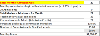
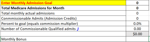
I need fillable cells to put "monthly goal" and "qualified admits" and then allow the formulas to take it from there. I am struggling because of the way the structure is based on % to goal rather than you hit x number and your payout equals y. If someone could help me with these formulas I would be forever grateful! I have browsed through the other threads and found questions that are close but not quite what I am looking for. The table I am currently working with looks like:

Thank you so much for your help!

 

[Dave Patton]

If you want the calculation on 22+1 , review the following

T202107a.xlsm
	A	B	C	D	E	F
1	Goal	20
2	Achieved	22			1.0	75
3		1			1.2	100
4	Amount	1,725.00	1,725.00		1.4	150
5					1.6	175
6					1.8	200
7
2e

Cell Formulas
Range	Formula
B4	B4	=(B2+B3)*LOOKUP((B2+B3)/B1,E2:F6)
C4	C4	=SUM(B2:B3)*LOOKUP(SUM(B2:B3)/B1,{1,75;1.2,100;1.4,150;1.6,175;1.8,200})

or

T202107a.xlsm
	A	B	C
1	Goal	20
2	Achieved	22
3		1
4		23
5	Amount	1,725.00	1,725.00
6
2e

Cell Formulas
Range	Formula
B4	B4	=SUM(B2:B3)
B5	B5	=B4*LOOKUP(B4/B1,E2:F6)
C5	C5	=B4*LOOKUP(B4/B1,{1,75;1.2,100;1.4,150;1.6,175;1.8,200})

What lookup table are you using?
What are your formulas?

 

[Jryan582]

Sir- I am using =B10*LOOKUP(B13/B9,E14:F23) as the formula for cell B14 and the lookup table is:

 

[Dave Patton]

Why did you change the Lookup table?
Did you change the definitions and rules for the calculations?
Is The formula that you showed yielding the result that you require?

 

[Jryan582]

Why did you change the Lookup table?
Did you change the definitions and rules for the calculations?
Is The formula that you showed yielding the result that you require?

My counterpart had mentioned that we needed to account for someone hitting 110%, 130%, 150% and 170%. I didnt change the definitions or rules I just copy and pasted what you had put together. No unfortunately what we have as the formula right now is not yielding the correct results.

 

[Dave Patton]

Unless you provide information, I cannot help.

 

[Jryan582]

Unless you provide information, I cannot help.

What information do you need?

 

[Dave Patton]

You could have posted the information with the forum's too XL2BB.

What formula did you use?
Why did you change the Lookup Table?
What is the complete description of what you want calculated?
What is the result if the goal is not attained?
Show some sample calculations with correct amounts.

 

[Jryan582]

You could have posted the information with the forum's too XL2BB.

What formula did you use?
Why did you change the Lookup Table?
What is the complete description of what you want calculated?
What is the result if the goal is not attained?
Show some sample calculations with correct amounts.

GHH NEW Calculator.xlsx
	I
11
Sheet2

Im not sure if I did that right or not, tried following the directions. The formula that I used was the one that was provided, I thought: =B10*LOOKUP(B13/B9,E14:F23)
I just added a few more items in the lookup table hoping that would be able to help the formula calculate payouts for a rep that hit in between the 100,120,140,160 and 180% ranges.

If the result is not attained the payout is zero, if the rep does not hit at least hit 100% of their budget there is no payout.

The calculation I was trying to work with is one where a rep achieves 23 on a goal of 20 or 115% which pays out at $75 per admit so it should work out to be $1725.00 but for some reason the formula is calculating it at 71% or a $1650 payout.

 

[Jryan582]

GHH NEW Calculator.xlsx
	A	B	C	D	E	F
4
5
6
7
8
9	Monthly Medicare Admission Goal	20
10	Medicare Admissions for the Month	22
11	LUPAs	1
12	Episodic Payer Admits **only if goal achieved, calculate at .5 per admit**	2
13	Total Admissions	23
14	Commission Payout	1650	1650
15					1	75
16					1.1	75
17					1.2	100
18					1.3	100
19					1.4	150
20					1.5	150
21					1.6	175
22					1.7	175
23					1.8	200
Sheet2

Cell Formulas
Range	Formula
B13	B13	=SUM(B10,B12)-B11
B14	B14	=B10*LOOKUP(B13/B9,E14:F23)
C14	C14	=B10*LOOKUP(B10/B9,{1,75;1.2,100;1.4,150;1.6,175;1.8,200})

 

[Dave Patton]

Your formula references the incorrect cell.

You can copy the post to a clean sheet and use Excel's Formula Evaluate to review the formula.

You did not post an extract of your sheet or answer the questions!!!

T202107a.xlsm
	A	B	C	D	E	F
1
2					1.0	75
3					1.2	100
4					1.4	150
5					1.6	175
6					1.8	200
7
8
9	Goal	20
10
11
12
13	Attained	23
14		1725
5c

Cell Formulas
Range	Formula
B14	B14	=IFERROR(B13*LOOKUP(B13/B9,E1:F6),"")