Data Comparison

Redgirl9487

New Member
Joined
Jan 18, 2023
Messages
9
Office Version
  1. 365
Platform
  1. Windows
Hey,

I was wondering if someone could me please?

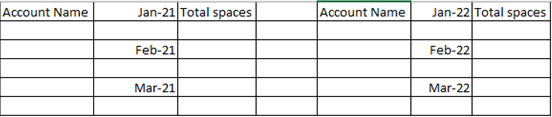
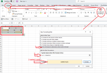
I have to summarise client data per month and compare that data for 2021 Vs 2022 So it reads something like image 1.

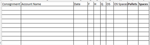
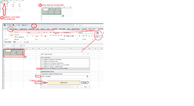
I have a large data dump, but I have split it into tab 1 which is the data for 2021 & tab 2 which is the data for 2022

Image 2 is an example of how the data table is.

Please could someone advise the best way to go about this?

I would appreciate anyone's help as I am a new excel user :)

Many thanks in advance.
 

Attachments

  • Image 1.png
    Image 1.png
    14.8 KB · Views: 9
  • Image 2.png
    Image 2.png
    18.5 KB · Views: 9

Excel Facts

Select all contiguous cells
Pressing Ctrl+* (asterisk) will select the "current region" - all contiguous cells in all directions.
It looks like 2 pivot tables will better suit your needs. You can filter the first one according to 2021 and the other according to 2022.
 
Upvote 0
Try this: This will compare data between tabs in same workbook:
  • n the worksheet where you want to highlight differences, select all used cells. For this, click the upper left cell of the used range, usually A1, and press Ctrl + Shift + End to extend the selection to the last used cell.
  • On the Home tab, in the Styles group, click Conditional Formatting > New rule, and create a rule with the following formula:
    =A1<>Sheet2!A1
  • It will highlighted the difference
 

Attachments

  • Sample comparison.png
    Sample comparison.png
    25.3 KB · Views: 4
Upvote 0
Or: use this formula:
To compare two Excel worksheets for differences, just open a new empty sheet, enter the following formula in cell A1, and then copy it down and to the right by dragging the fill Handle:

=IF(Sheet1!A1 <> Sheet2!A1, "Sheet1:"&Sheet1!A1&" vs Sheet2:"&Sheet2!A1, "")
 

Attachments

  • Test Sample.png
    Test Sample.png
    23.8 KB · Views: 3
Upvote 0
Try this: This will compare data between tabs in same workbook:
  • n the worksheet where you want to highlight differences, select all used cells. For this, click the upper left cell of the used range, usually A1, and press Ctrl + Shift + End to extend the selection to the last used cell.
  • On the Home tab, in the Styles group, click Conditional Formatting > New rule, and create a rule with the following formula:
    =A1<>Sheet2!A1
  • It will highlighted the difference
Thanks! Please could you confirm what rule type I would select please? Many thanks in advance.
 
Upvote 0
See attached:
1- Use a formula to determine which cell to format
2- enter formula: =A1<>Sheet2!A1
3- Select the Pattern Color

Hope this will help?
 

Attachments

  • Sample comparison1.png
    Sample comparison1.png
    52.6 KB · Views: 5
Upvote 0
See attached:
1- Use a formula to determine which cell to format
2- enter formula: =A1<>Sheet2!A1
3- Select the Pattern Color

Hope this will help?
Thanks. For some reason it does not seem to work. I have copied your formula into a new sheet however, no data information is being pulled from the sheets named 2021 and 2022.
 
Upvote 0
You must select sheet1.
Select A1 on sheet 1 then press: Ctrl+Shift+End so it will select the entire data then use format conditions and the formula
 
Upvote 0
It looks like 2 pivot tables will better suit your needs. You can filter the first one according to 2021 and the other according to 2022.
Thanks. Please could you advise how I would create a pivot table?
 
Upvote 0
Follow the steps as per attachment below:
 

Attachments

  • Comparison data.png
    Comparison data.png
    72 KB · Views: 10
Upvote 0

Forum statistics

Threads
1,216,434
Messages
6,130,611
Members
449,584
Latest member
c_clark

We've detected that you are using an adblocker.

We have a great community of people providing Excel help here, but the hosting costs are enormous. You can help keep this site running by allowing ads on MrExcel.com.
Allow Ads at MrExcel

Which adblocker are you using?

Disable AdBlock

Follow these easy steps to disable AdBlock

1)Click on the icon in the browser’s toolbar.
2)Click on the icon in the browser’s toolbar.
2)Click on the "Pause on this site" option.
Go back

Disable AdBlock Plus

Follow these easy steps to disable AdBlock Plus

1)Click on the icon in the browser’s toolbar.
2)Click on the toggle to disable it for "mrexcel.com".
Go back

Disable uBlock Origin

Follow these easy steps to disable uBlock Origin

1)Click on the icon in the browser’s toolbar.
2)Click on the "Power" button.
3)Click on the "Refresh" button.
Go back

Disable uBlock

Follow these easy steps to disable uBlock

1)Click on the icon in the browser’s toolbar.
2)Click on the "Power" button.
3)Click on the "Refresh" button.
Go back
Back
Top