Data Validation List - Not Including Blanks

[jbodel]

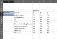
I have a data Validation List that is based off another cell. If that one cell says A it will list all the services listed for A, but if they select B, it will list all the services for B. The list is alphabetized, and some services might be used with multiple different selections. Right now when you select that Cell (A) it will have a list but have a long scroll where there are blanks. Is there a way to avoid that?

 

[Jeffrey Mahoney]

Please consider this. Multiple Criteria can be used in the Filter Function. See where I filtered for Letter B AND for Numbers that weren't blank. Your criteria's must be surrounded by parenthesis to work.

Book1
	H	I	J	K
6	Filter		Letters	Numbers
7	10		A	1
8	11		B	10
9	13		A	2
10			B	11
11			C
12			B
13			A	3
14			B	13
15			C	23
Sheet2

Cell Formulas
Range	Formula
H7:H9	H7	=FILTER(K7:K15,(J7:J15="B")*(K7:K15<>""),"")
Dynamic array formulas.

 

[jbodel]

Thank you so much for your help. I am not sure I explained it correctly. So in the example, if they select A, the drop down would show everything marked with a yes (but listing the services). So anything listed with a NO would not be listed and there would be no spaces. Does that make more sense?

 

[Jeffrey Mahoney]

Well it would have been nice for you to lead with that. I can help you. Is there any way you can post that using XL2BB so I don't have to type it out?

 

[jbodel]

I can, but it might be a bit. Using my work computer and they don't allow any downloads. Let me transfer to my personal computer. Sorry about the missed information. Thanks in advance for any help I really appreciate it.

 

[kevin9999]

Not sure where you want your actual data validation list to appear, but does this give you what you want? When you select A, B or C in cell A6, the filtered services will appear in A7, and the data validation list in cell A2 will change accordingly. Don't know how many services you'll have listed, I allowed for 95 - increase if needed.

Book1
	A	B	C	D	E
1	Data Validation List Below
2
3
4
5	Selection	Service	A	B	C
6	A	Checking Account	Yes	Yes	No
7	Checking Account	Savings Account	Yes	No	No
8	Savings Account	CD	Yes	No	No
9	CD	Loan	Yes	Yes	No
10	Loan	Commercial Checking Account	No	No	No
11	Credit Card
12	Debit Card	Kids Checking Account	No	No	No
13		Home Equity Loan	No	No	No
14		Credit Card	Yes	No	Yes
15		Debit Card	Yes	No	Yes
Sheet1

Cell Formulas
Range	Formula
A7:A12	A7	=CHOOSECOLS(FILTER(B6:E100,(B6:B100<>"")*(OFFSET(B5,1,MATCH(A6,C5:E5,0),95,1)="Yes")),1)
Dynamic array formulas.

Cells with Data Validation
Cell	Allow	Criteria
A6	List	=$C$5:$E$5
A2	List	=$A$7#

 

[jbodel]

Kevin

I have to admit that it looks like what you wrote is going to work and I have tried to re-create it. I am not 100% an excel expert by any means, but I am a bit confused when you when you in your instructions said Range (A78:A12) Where do I Put that and how? I have tried to do everything else, but not getting it to work.

Jeffrey - I also want to thank you as well. I unfortunately could not get that XL2BB to download. Again sorry not super techie either.

Apologize to both of you for the delay in responding. Busy weekend. Thank you in advance.

Not sure where you want your actual data validation list to appear, but does this give you what you want? When you select A, B or C in cell A6, the filtered services will appear in A7, and the data validation list in cell A2 will change accordingly. Don't know how many services you'll have listed, I allowed for 95 - increase if needed.

Book1
	A	B	C	D	E
1	Data Validation List Below
2
3
4
5	Selection	Service	A	B	C
6	A	Checking Account	Yes	Yes	No
7	Checking Account	Savings Account	Yes	No	No
8	Savings Account	CD	Yes	No	No
9	CD	Loan	Yes	Yes	No
10	Loan	Commercial Checking Account	No	No	No
11	Credit Card
12	Debit Card	Kids Checking Account	No	No	No
13		Home Equity Loan	No	No	No
14		Credit Card	Yes	No	Yes
15		Debit Card	Yes	No	Yes
Sheet1

Cell Formulas
Range	Formula
A7:A12	A7	=CHOOSECOLS(FILTER(B6:E100,(B6:B100<>"")*(OFFSET(B5,1,MATCH(A6,C5:E5,0),95,1)="Yes")),1)
Dynamic array formulas.

Cells with Data Validation
Cell	Allow	Criteria
A6	List	=$C$5:$E$5
A2	List	=$A$7#

Not sure where you want your actual data validation list to appear, but does this give you what you want? When you select A, B or C in cell A6, the filtered services will appear in A7, and the data validation list in cell A2 will change accordingly. Don't know how many services you'll have listed, I allowed for 95 - increase if needed.

Book1
	A	B	C	D	E
1	Data Validation List Below
2
3
4
5	Selection	Service	A	B	C
6	A	Checking Account	Yes	Yes	No
7	Checking Account	Savings Account	Yes	No	No
8	Savings Account	CD	Yes	No	No
9	CD	Loan	Yes	Yes	No
10	Loan	Commercial Checking Account	No	No	No
11	Credit Card
12	Debit Card	Kids Checking Account	No	No	No
13		Home Equity Loan	No	No	No
14		Credit Card	Yes	No	Yes
15		Debit Card	Yes	No	Yes
Sheet1

Cell Formulas
Range	Formula
A7:A12	A7	=CHOOSECOLS(FILTER(B6:E100,(B6:B100<>"")*(OFFSET(B5,1,MATCH(A6,C5:E5,0),95,1)="Yes")),1)
Dynamic array formulas.

Cells with Data Validation
Cell	Allow	Criteria
A6	List	=$C$5:$E$5
A2	List	=$A$7#

 

[kevin9999]

I am a bit confused when you when you in your instructions said Range (A78:A12)

Sorry but - where did I say that?

 

[jbodel]

Sorry but - where did I say that?

When you gave the instructions under the spreadsheet you said Cell Formula's. Range - Formula. You gave the formula that I need to put in cell A7, but what about the Range that you reference to the left? That is where I am struggling.

 

[jbodel]

When you gave the instructions under the spreadsheet you said Cell Formula's. Range - Formula. You gave the formula that I need to put in cell A7, but what about the Range that you reference to the left? That is where I am struggling.

Sorry I referenced (A78:A12). I meant to say A7:A12