Multiple Conditional Data Validations

[Nathan Asius]

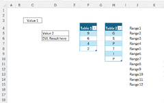
I am attempting to insert various Validation lists in Cell D6 based upon Multiple conditions.
I have a Data Validation List from Table 1 in C3. And another Data Validation List from Table 2 in D6.
Whichever of the multiple AND conditions appear from those many permutations I would like any of the specific Data Validation Lists Defined with the multiple range names on the right show up.

I was beginning to enter in a very long IF(AND nested formula in my List box for cell D6 until I realized how long it would be before I lost track. I tried mapping it out on paper and speculated there must be a better way.
I looked up using Case Statements (VBA) realizing it is not ideal for this task either.

Any suggestions on the most efficient way to do this? Excel 365.

Thanks,
Nathan

 

[dreid1011]

Could you provide some sample data and expected results please?

I am assuming you combine the values from each DV to get your final result... from the values in column J? Can you explain how the combinations work to determine results?

 

[Nathan Asius]

Yes you're correct that combining values from each DV gives me the result
Column J contains names ranges which will populate the Data Validation List I want as my result in D6. Each named range will have varying number of entries.
So if in cell C3 "9" is selected and also in D5 "G is selected then in D6 a specific data validation list from Range1 displays. The User will select options from either cell.
Any combination from both C3 and D5 can be possible.

 

[Nathan Asius]

......Here is an example of the nested formula I was trying to place in the Data Validation dialog box:

=IF(AND(C3="9",D5="G"),G9,IF(AND(C3="9",D5="S"),S9,IF(AND(C3="6",D5="G"),G6,IF(AND(C3="6",D5="S"),S6,IF(AND(C3="4",D5="G"),G4,IF(AND(C3="4",D5="S"),S4,IF(AND(C3="4",D5="T"),T4,IF(AND(C3="4",D5="P"),P4,W2)…….. )))))))

I think this demonstrates that there are two many permutations to accomplish this with a formula. There must be a better designed function or solution to do this.

Thanks,

 

[dreid1011]

......Here is an example of the nested formula I was trying to place in the Data Validation dialog box:

=IF(AND(C3="9",D5="G"),G9,IF(AND(C3="9",D5="S"),S9,IF(AND(C3="6",D5="G"),G6,IF(AND(C3="6",D5="S"),S6,IF(AND(C3="4",D5="G"),G4,IF(AND(C3="4",D5="S"),S4,IF(AND(C3="4",D5="T"),T4,IF(AND(C3="4",D5="P"),P4,W2)…….. )))))))

I think this demonstrates that there are two many permutations to accomplish this with a formula. There must be a better designed function or solution to do this.

Thanks,


View attachment 105339

What do the combinations point to? If the combination is G9, what is the end result?

 

[Nathan Asius]

G9, or S9 etc.. are just the shorthand of the named ranges that the DV list pulls from. I see now that it actually might make you think it's a cell reference.
So the column on the right in my attached image was very generic. But the example of the formula demonstrates my ranges to have names.

 

[dreid1011]

G9, or S9 etc.. are just the shorthand of the named ranges that the DV list pulls from. I see now that it actually might make you think it's a cell reference.
So the column on the right in my attached image was very generic. But the example of the formula demonstrates my ranges to have names.

Ok, so lets walk through this step by step.

If I select "9" for value 1, and "S" for value 2, this represents a named range called "S9". (Could these two lists be swapped so value 1 is the letter and value 2 is the number?)

In cell D6, should it just display the combination of values 1 and 2? Or is something else supposed to happen?

Now that we have the name of the range, what is supposed to happen with the named range? Do you want a third data validation list to show values contained in the named range?

 

[Nathan Asius]

Ok, so lets walk through this step by step.

If I select "9" for value 1, and "S" for value 2, this represents a named range called "S9". (Could these two lists be swapped so value 1 is the letter and value 2 is the number?)

In cell D6, should it just display the combination of values 1 and 2? Or is something else supposed to happen?

Now that we have the name of the range, what is supposed to happen with the named range? Do you want a third data validation list to show values contained in the named range?

You got some of that correct. Yes. selecting '9' for the first value in cell C3, and selecting 's' for value 2 in cell d5 represents a named range in a hidden worksheet elsewhere.
However, value 1 and value 2 should not be switched. You can't get the same list where 9 occurs as a choice in cell D5 and vice versa.
Remember, I originally wanted the sample formula accounting for all the permutations of options to be entered in the Data Validation Box.
So that means, I aim for Cell D6 to produce a dependent List based on the selection of C3 and D5. So yes, a third data validation list would be displayed. And many more lists displayed on every other possible combination of choices.

 

[dreid1011]

You got some of that correct. Yes. selecting '9' for the first value in cell C3, and selecting 's' for value 2 in cell d5 represents a named range in a hidden worksheet elsewhere.
However, value 1 and value 2 should not be switched. You can't get the same list where 9 occurs as a choice in cell D5 and vice versa.
Remember, I originally wanted the sample formula accounting for all the permutations of options to be entered in the Data Validation Box.
So that means, I aim for Cell D6 to produce a dependent List based on the selection of C3 and D5. So yes, a third data validation list would be displayed. And many more lists displayed on every other possible combination of choices.

And by looking at your formula, all it seems you are doing is putting the letter before the number. Or am I missing something you haven't explained yet?

 

[Nathan Asius]

OK. I'm coming back to this attempting to make things clearer of what I'm aiming to do.
Basically I'm looking to create dependent Drop Down Lists. I created a sample table here that makes things very self explanatory. I know that these dependent drop down lists can be created within the same contiguous range or a table using the indirect function. Where the sample table helps is to be able to see the columns and lists in a successional flow from left to right. Each list is a named range pertaining to the column header.
In cell C16, I have a drop down list, To create this as a dependent list, I'm entering this formula in the Validation List Window:
=IF($B$16=$B$3,One,IF($B$16=$B$4,Two,IF($B$16=$B$5,Three,IF($B$16=$B$6,Four,IF($B$16=$B$7,Five)))))
My struggle is not understanding how the Indirect and Substitute functions work. Because if I'm trying to make a dependent list from every possible combination that could occur with this table, I don't know how to build that.
But as I said, this table helps cause I can show it all at one glance. My bigger difficulty is that all of my lists/named ranges are from various worksheets, tables and ranges (all named though).
How can I build a multi-dependent series of dropdown lists from many different areas in my workbook?