Data Validation list to have a certain value

[craigwojo]

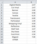
In a Data Validation cell, I need to have a value for each item. If they pick "Digital Media" in E3 then the value would be 1.50. The items associated with the cell are (=Sheet2!A1:A14).
How is this done?

 

[jasonb75]

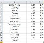
From the way your question is phrased, it suggests that you want to have the value entered into the cell with the validation dropdown which is not possible, you would need a vlookup formula in the next cell to look for the dropdown selection in sheet2 column A, then return the corresponding value in sheet2 column B.

 

[craigwojo]

This is what I have on Sheet 2. New to this, so what should I do.

 

[jasonb75]

So the dropdown is in E3? If so then in F3,

=VLOOKUP(E3,Sheet2!$A$1:$B$14,2,0)

Note that it will return 0 if E3 contains 'Other'. If you overtype the formula with a value when that happens, the formula will be gone unless you re-enter it again afterwards. It will not be replaced automatically next time you change the dropdown.

 

[craigwojo]

So the dropdown is in E3? If so then in F3,

=VLOOKUP(E3,Sheet2!$A$1:$B$14,2,0)

Note that it will return 0 if E3 contains 'Other'. If you overtype the formula with a value when that happens, the formula will be gone unless you re-enter it again afterwards. It will not be replaced automatically next time you change the dropdown.

You're the best Jason.
Thank you.

 

[craigwojo]

I have another cell that needs the same VLOOKUP but the column is "C" instead of "B", how is this done?
The formula cell would be "R3"

 

[jasonb75]

Like this,

=VLOOKUP(E3,Sheet2!$A$1:$C$14,3,0)

What you're looking for, e.g. the dropdown must always be in the column on the left. You can have as many columns as you need. The number, 3 in the formula above is the column where the result should be taken from.

The 0 at the end tells the formula that it must find an exact match for the criteria (the dropdown).

 

[craigwojo]

In K3 I need to add .20 per sqft if "YES' is chose (=Sheet2!$D$1:$D$3) the cell that contains "YES" is D2.

Also, if L3 is "YES" it will add 10% to N3 and P3.

 

[jasonb75]

This part is a little unclear

In K3 I need to add .20 per sqft if "YES' is chose (=Sheet2!$D$1:$D$3) the cell that contains "YES" is D2.

Are you saying if K3="YES" then N3 should be $8.20 (in the example)?

What formulas do you already have in N3 and P3?

 

[craigwojo]

Yes. Easy, but I don't know how to make an input with data validation to be added to another cell.

Thank you once again.