dadodagrisez
New Member
- Joined
- Aug 9, 2023
- Messages
- 3
- Office Version
- 2021
Hello,
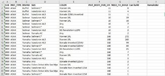
This report has been taking me hours to do every month. Here is my challenge. In each of our Warehouse locations we have a set number of Instruments that need to be distributed to a number of orders we have for that instrument. Here is what each column represents:
A: The warehouse location number
B: The type of Instrument
C: The Brand of Instrument
D & E: Are not relevant to what I am wanting to accomplish
F: The total number of that brand of instrument
G: The number of instruments that need to be built for each order.
H & I: Is where I am hoping to put the formulas that can make this report easier
Take rows 2-4 as an example. I have enough materials to build 11 of the Buffet Saxophones. I need 8 for one order, 4 for the next order, and 1 for the last order. I want to fulfill these orders by the greatest amount needed to the least. So I can fulfill the first order of 8 (cell H2). Which would leave me with 3 left (Cell I2). I can build then 3 out of 4 for the second order so 3 (cell H3) and 0 (Cell I3). Then I have none for the third order so 0 (Cell H4 and I4). As you can see, I have multiple orders per location, and I have multiple locations as well. Any help on this would be awesome.
Thanks,
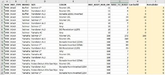