Detect peak maximum on a spectrum from the raw data

mejohn

New Member
Joined
Jun 23, 2018
Messages
31
Office Version
  1. 365
Platform
  1. Windows
Hello everyone!
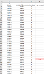
I’m trying to detect a peak maximum from the raw data of a spectrum, but only if the peak rises and falls by a minimum amount.

The formula I currently have will detect this, but only on sharp peaks which rise and fall by the minimum amount between adjacent row values.
So, if B10-B9>=positive minimum value AND B11-B10<=negative minimum value, then the peak is detected.
But if the peak is shallow, then the difference between adjacent row values is smaller than the minimum, and the peak will not be detected.

Here’s the main formula on Column E
=IFERROR(IF(((B10-B9)/($A9-$A10))>0,IF(AND((B9-B8)/($A8-$A9)>0,(B10-B8>=0.0006),(B11-B10<=-0.0006)),"True",""),""),"")

Columns C and D are not used in the formula, they only inform if the difference between adjacent row values are positive (peak rise) or negative (peak fall). Column D shows this in 1's (rise) and 0's (fall).

I’d like to account for all the consecutive peak rises (positive values on Column C) after a peak fall (negative values on Column C), and determine if the difference between the start of the peak rise and it’s fall is >=0.0006
At the same time, account for all consecutive peak falls (negative values) after a peak rise, and determine if the difference between the start of the peak fall and the start of the next peak rise is <=-0.0006
If both of these conditions are met, then report "True", as a peak was detected.

I hope this makes sense. Thank you all in advance for your time!

1661962137610.png
 

Attachments

  • peak detection.png
    peak detection.png
    24.1 KB · Views: 5
Hi Peter,

The new formula works perfectly!

Thank you so much for your help!
 
Upvote 0

Excel Facts

Which came first: VisiCalc or Lotus 1-2-3?
Dan Bricklin and Bob Frankston debuted VisiCalc in 1979 as a Visible Calculator. Lotus 1-2-3 debuted in the early 1980's, from Mitch Kapor.
The new formula works perfectly!
I am having second thoughts.
So, just checking, should the yellow cell below show 'True'?

mejohn.xlsm
ABCD
1Wavelength (nm)APeak Detected
25000.000056
34990.0000711 
4498-0.0000630 
5497-0.0000750 
64960.0000711 
7495-0.0000630 
8494-0.0000750 
9493-0.0006820 
10492-0.0000171 
11491-0.0007370 
12490-0.0007361 
Sheet7
Cell Formulas
RangeFormula
C3:C12C3=(C2+1)*(B3>B2)
D3:D12D3=IF(OR(C3=0,C4>0),"",IF(MIN(B3-XLOOKUP(1,C$2:C2,B$2:B2,0,0,-1),B3-XLOOKUP(1,C4:C$100,B3:B$99,B$99))>=0.0006,"True",""))
 
Upvote 0
Hi Peter,
That data seems to be a subset of the data I provided.
But using the data you presented, yes, 492 should be a peak maximum and reflected as "True"
B10-B9 = 0.000665 (which is >=0.0006)
B11-B10 = -0.00072 (which is <=-0.0006)

Good catch!
 
Upvote 0
That data seems to be a subset of the data I provided.
Sort of - I fudged some of the numbers to produce that single "1" with surrounding values that I though might trigger a 'True'

However, before I consider a formula modification, it may be that the logic of the existing formula is not quite correct & I would like that checked.
When we think that we might have a peak, we have to check upwards to ensure >=0.0006 and we have to check downwards for <=-0.0006. Is that correct?

If so, when looking at row 39 in the sample below ..
When checking upwards, should I be checking the difference between yellow and blue or should I be checking between yellow and green to confirm >=0.0006?

Similarly, what about when checking downwards?

My existing formula is comparing blue upwards and green downwards which is probably not correct? Should it be green in both directions? .. or something else?

mejohn.xlsm
ABCD
254770.000040 
264760.0000521 
274750.0001542 
284740.000243 
294730.0003934 
304720.000575 
314710.0009096 
324700.0014727 
334690.0022178 
344680.003569 
354670.0059910 
364660.01075411 
374650.01766512 
384640.02418213 
394630.02664514True
404620.0257080 
414610.0248940 
424600.0249551 
Sheet7
Cell Formulas
RangeFormula
C25:C42C25=(C24+1)*(B25>B24)
D25:D42D25=IF(OR(C25=0,C26>0),"",IF(MIN(B25-XLOOKUP(1,C$2:C24,B$2:B24,0,0,-1),B25-XLOOKUP(1,C26:C$100,B25:B$99,B$99))>=0.0006,"True",""))
 
Upvote 0
Hi Peter,

Yes, "we have to check upwards to ensure >=0.0006 and we have to check downwards for <=-0.0006"

For row 39, the peak fall is calculated by subtracting B41-B39, so green minus yellow.
This is because after peak maximum at row 39, the peak falls from its maximum 39 to row 41. In this case, the total fall from row 39 to 41 (B41-B39) needs to be <=-0.0006.
Between row 41 and row 42, the peak (absorbance) starts going back up, so row 42 would not be included as a peak fall.
Also B42-B41 would be included in the calculation of a peak rise, if there was more data after row 42.

Thank you so much for being diligent and accurate with the calculations.
 
Upvote 0
For row 39, the peak fall is calculated by subtracting B41-B39, so green minus yellow.
Thanks, but that is for the downwards check only. You didn't clarify for the upwards check. :)
Should it be B39-B26 (blue) or B39-B25 (green)?
 
Upvote 0
Hi Peter,
Sorry, I missed that.
The peak rise for peak maximum at wavelength 463 should be calculated by B39-B25, yellow-green.
Thank you!
 
Upvote 0
The peak rise for peak maximum at wavelength 463 should be calculated by B39-B25, yellow-green.
Thanks. That means my previous formula was incorrect with its 'upwards' check. Try this instead.

mejohn.xlsm
ABCD
1Wavelength (nm)APeak Detected
25000.000056
34990.0000711 
4498-0.0000630 
5497-0.0000750 
64960.0000711 
7495-0.0000630 
8494-0.0000750 
9493-0.0006820 
10492-0.0000171True
11491-0.0007370 
12490-0.0007361 
13489-0.0000642 
14488-0.0000023 
15487-0.0001060 
16486-0.000041 
174850.0000652 
18484-0.0000180 
194830.0000841 
20482-0.0000170 
21481-0.0000151 
2248002 
23479-0.0000450 
244780.0000511 
254770.000040 
264760.0000521 
274750.0001542 
284740.000243 
294730.0003934 
304720.000575 
314710.0009096 
324700.0014727 
334690.0022178 
344680.003569 
354670.0059910 
364660.01075411 
374650.01766512 
384640.02418213 
394630.02664514True
404620.0257080 
414610.0248940 
424600.0249551 
434590.0256872 
444580.0282083 
454570.0318994 
464560.034345 
474550.0346126True
484540.0334980 
494530.0313120 
76426-0.0044660 
77425-0.0042581 
78424-0.0032622 
79423-0.000983 
804220.0035084 
814210.0119295 
824200.0263536 
834190.0494817 
844180.0847638 
854170.1353649 
864160.20323310 
874150.28807711 
884140.38454312 
894130.48809213 
904120.60167214 
914110.72905515 
924100.86149516 
934090.97718117 
944081.05993718 
954071.11896319 
964061.16586120 
974051.20055921 
984041.21490922True
994031.2135580 
Sheet8
Cell Formulas
RangeFormula
C3:C49,C76:C99C3=(C2+1)*(B3>B2)
D3:D49,D76:D99D3=IF(C3>C4,IF(MIN(B3-XLOOKUP(1,C$3:C3,B$2:B2,0,0,-1),B3-XLOOKUP(1,C4:C$100,B3:B$99,B$99))>=0.0006,"True",""),"")
 
Upvote 0
Solution
Hi Peter,

I made manual modifications to the data to better test the formula and found that the latest or previous formulas fail to detect a peak at row 352 (wavelength 457) in the data below.

Thanks!

Appendix B_Template Methanol.xlsx
ABCDL
345464-0.0001660 
346463-0.0001371 
347462-0.000150 
348461-0.0001491 
349460-0.0001412 
350459-0.000143 
351458-0.0001014 
3524570.0004555 0.00061
353456-0.0000860 -0.00060
354455-0.0000960 
355454-0.00010 
356453-0.0001030 
357452-0.000140 
358451-0.0001440 
359450-0.0001171 
360449-0.0001112 
Raw Data Combined
Cell Formulas
RangeFormula
C345:C360C345=(C344+1)*(B345>B344)
D345:D360D345=IF(C345>C346,IF(MIN(B345-XLOOKUP(1,C$10:C345,B$9:B344,0,0,-1),B345-XLOOKUP(1,C346:C$600,B345:B$599,B$599))>=0.0006,"True",""),"")
L352L352=B352-B347
L353L353=B358-B352
Cells with Conditional Formatting
CellConditionCell FormatStop If True
D10:D599Cell Valuecontains "True"textNO
 
Upvote 0
I don't believe that row 352 is a peak. Your values in column L (as shown) are incorrect. If you physically look at B358, the 6th decimal place is a 4. For B352 the 6th decimal place is a 5. So subtracting them can not leave a zero in the 6th decimal place as "appears" (or does not appear) in cell L353. I suspect that you have column L set to display 5 decimal places only?

If you manually do that subtraction, the result is -0.000599 which is not <=-0.0006 hence no peak.
(L352 is also different. The actual value is 0.000605 but is this case it doesn't 'flip' the result to the other side of >=0.0006 so no harm done)

Having said all that, I cannot guarantee that a peak will not be missed, or an extra peak could get included due to the fact that calculating in Excel is not always perfect.
See Floating-point arithmetic may give inaccurate result in Excel - Office
 
Upvote 0

Forum statistics

Threads
1,216,079
Messages
6,128,687
Members
449,464
Latest member
againofsoul

We've detected that you are using an adblocker.

We have a great community of people providing Excel help here, but the hosting costs are enormous. You can help keep this site running by allowing ads on MrExcel.com.
Allow Ads at MrExcel

Which adblocker are you using?

Disable AdBlock

Follow these easy steps to disable AdBlock

1)Click on the icon in the browser’s toolbar.
2)Click on the icon in the browser’s toolbar.
2)Click on the "Pause on this site" option.
Go back

Disable AdBlock Plus

Follow these easy steps to disable AdBlock Plus

1)Click on the icon in the browser’s toolbar.
2)Click on the toggle to disable it for "mrexcel.com".
Go back

Disable uBlock Origin

Follow these easy steps to disable uBlock Origin

1)Click on the icon in the browser’s toolbar.
2)Click on the "Power" button.
3)Click on the "Refresh" button.
Go back

Disable uBlock

Follow these easy steps to disable uBlock

1)Click on the icon in the browser’s toolbar.
2)Click on the "Power" button.
3)Click on the "Refresh" button.
Go back
Back
Top