Different formulas based on a value

Fantrasp12

New Member
Joined
Jan 14, 2023
Messages
8
Office Version
  1. 365
  2. 2021
Platform
  1. Windows
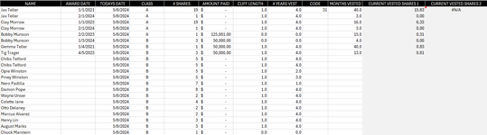
Hi, so I'm having a relaly hard time here. I'm building a cap table (shares vesting) but based on different scenarios. For example, 4 years with 1 year cliff (and no cliff), 3 years with 1 year cliff, and so on. I have all the different formulas working independently, but i don't want people in my company to have to choose and manually copy/paste a formula each time (will confuse people and prone to error). Ideally i can just have a code in a cell that represents what formula to use. For example, you can see in the exhibit below, The formulas work in column N, example =IF(DATEDIF(E2,F2,"D")<365,0,MIN(DATEDIF(E2,F2,"M")/48*H2,H2)), but this is based only on a 48 month vesting schedule with no cliff. I did try to make 2 arguments with 36 and 48 month vesting with an IF using the code in column L to read from (see formula exhibited below which represents O2, But, it doesnt work. I either get "FALSE" if i use "IFS", i get invalid if i use "IF", and i've tried so many combinations of parenthesis that won't make it work. I've also tried "CHOOSE function, to no avail. I suspect its the nested arguments within one another that need more nuance.

FYI, so it will be a pretty long formula given the scenarios i have to cover. For example:

1715216836970.png


1715214793106.png
 

Attachments

  • 1715214755750.png
    1715214755750.png
    73.9 KB · Views: 0

Excel Facts

How to create a cell-sized chart?
Tiny charts, called Sparklines, were added to Excel 2010. Look for Sparklines on the Insert tab.
One way, which I think would be better for maintenance than a very long and complex formula, would be to make use of some of the sheet real estate to calculate every value in a separate column, and then use HLOOKUP to get the correct answer by looking up the code. You could even put the calculations on another sheet and hide it if you really wanted.

Like so:
Book1
DEFGHIJKLMNOPQ
1Award dateToday's date# SharesCodeCurrent Vested3141
21/01/20218/05/20241931191915.83
31/01/20218/05/2024194115.831915.83
Sheet1
Cell Formulas
RangeFormula
P2:P3P2=IF(DATEDIF(E2,F2,"D")<365,0,MIN(DATEDIF(E2,F2,"M")/36*H2,H2))
Q2:Q3Q2=IF(DATEDIF(E2,F2,"D")<365,0,MIN(DATEDIF(E2,F2,"M")/48*H2,H2))
N2:N3N2=HLOOKUP(L2,$P$1:$Q2,ROW(),FALSE)
 
Upvote 0
One way, which I think would be better for maintenance than a very long and complex formula, would be to make use of some of the sheet real estate to calculate every value in a separate column, and then use HLOOKUP to get the correct answer by looking up the code. You could even put the calculations on another sheet and hide it if you really wanted.

Like so:
Book1
DEFGHIJKLMNOPQ
1Award dateToday's date# SharesCodeCurrent Vested3141
21/01/20218/05/20241931191915.83
31/01/20218/05/2024194115.831915.83
Sheet1
Cell Formulas
RangeFormula
P2:P3P2=IF(DATEDIF(E2,F2,"D")<365,0,MIN(DATEDIF(E2,F2,"M")/36*H2,H2))
Q2:Q3Q2=IF(DATEDIF(E2,F2,"D")<365,0,MIN(DATEDIF(E2,F2,"M")/48*H2,H2))
N2:N3N2=HLOOKUP(L2,$P$1:$Q2,ROW(),FALSE)
Thanks. I'm not sure how that would exactly work though. My first effort was to do something like this but couldn't pull the formula in by using a code. I guess i could use a code to look the answer up. But i am trying to not burden the user to deal too much with where to enter codes, how it calculates (I'm not going to be the user). Are you saying that I would have another sheet that would just calculate all possible formulas and then the code would grab the one i want? If so I suppose this could work but seems like alot of work and use of real estate just to get one answer (and many that I don't need). Can you please conform this is the approach?

I think it would be much more compact and simpler to just find the answer right in the appropriate cell and avoid all unnecessary calculations and lookups. The formula is what i'm stuck on. I've done IFS, but the additional IF as part of the formula i think its not letting all arguments process from left to right completely. I'd appreciate thoughts on both approaches...thank you.
 
Upvote 0
The sheet I attached is an example of how to do it. All your user needs to know is the code to put in column L, which you could supply by a dropdown.
The “code” in my example is in columns P and Q (as a column header). The HLOOKUP formula in column N just takes the code value in column L, looks it up in P1:Q1 ( or more columns depending on how many formulas you have) and returns the answer.
The calculations in columns P and Q can be shifted to another sheet to hide them.
Post your other calculations and codes and I’ll send a link to an example spreadsheet.
 
Upvote 0
If you still want to go down the one formula route, then your IF statement is this (for just codes 31 and 41).

Excel Formula:
=IF(L2=31,IF(DATEDIF(E2,F2,"D")<365,0,MIN(DATEDIF(E2,F2,"M")/36*H2,H2)),IF(L2=41,IF(DATEDIF(E2,F2,"D")<365,0,MIN(DATEDIF(E2,F2,"M")/48*H2,H2)),"Undefined code"))
As you can see by the time you add another 7 formulas to this it's going to be pretty ugly.

A good way to approach it if you want to do this is to put each formula corresponding to each code in a cell, and then build the formula by referring to those cells initially. This will give you an intermediate step something like:
Excel Formula:
=IF(L2=31,P2,IF(L2=41,Q2,IF(L2=1A,<Formula if code is 1A>,"Message if no conditions are true")))
Once you have that working you can then copy/paste the respective formulas into their locations - for example, swap the formula in P2 for the reference to P2, giving:
Excel Formula:
=IF(L2=31,IF(DATEDIF(E2,F2,"D")<365,0,MIN(DATEDIF(E2,F2,"M")/36*H2,H2)),IF(L2=41,Q2,IF(L2=1A,<Formula if code is 1A>,"Message if no conditions are true")))
and so on.
 
Upvote 0
Solution
=IF(L2=31,IF(DATEDIF(E2,F2,"D")<365,0,MIN(DATEDIF(E2,F2,"M")/36*H2,H2)),IF(L2=41,IF(DATEDIF(E2,F2,"D")<365,0,MIN(DATEDIF(E2,F2,"M")/48*H2,H2)),"Undefined code"))
THANK YOU. I did initially tried to have formulas switch based on codes, but determined (after hours) this isn't possible. After hours of trying and researching seems cells don't know how to handle this, only pull in the actual values form those cells (not the formula). At least that's what I concluded. Are you saying tha tit is possible?

As fir the long formula, thank you!. Looks like you just added the "undefined code")) at the end? What does that do? I don't mind the long formula as opposed to having to build an enormous table of hundreds of cells instead (would have to repeat all of this for future quarterly projections).
 
Upvote 0
Are you saying tha tit is possible?
Yes, entirely possible.

Re the “undefined code”, every IF statement needs a TRUE clause and a FALSE clause. Since we are nesting multiple IF statements together, the last FALSE clause needs to handle the case where none of the preceding cases apply.
The actual text is irrelevant - it could say “pineapples” equally well.
 
Upvote 0
Yes, entirely possible.

Re the “undefined code”, every IF statement needs a TRUE clause and a FALSE clause. Since we are nesting multiple IF statements together, the last FALSE clause needs to handle the case where none of the preceding cases apply.
The actual text is irrelevant - it could say “pineapples” equally well.
thanks, i think i get lost in the multiple nested parts, and how things i've gotten to work in the past much harder in com plex scenarios.

Would you mind pointing me to a link that explains how to get formulas to switch using a code? I spent hours trying to do this and all info i came up with was either irrelevant or said it couldn't be done. I'd like to save you the trouble so am happy to dig in where this is already explained at a detailed level. Many thanks!!!
 
Upvote 0

Forum statistics

Threads
1,216,124
Messages
6,128,979
Members
449,480
Latest member
yesitisasport

We've detected that you are using an adblocker.

We have a great community of people providing Excel help here, but the hosting costs are enormous. You can help keep this site running by allowing ads on MrExcel.com.
Allow Ads at MrExcel

Which adblocker are you using?

Disable AdBlock

Follow these easy steps to disable AdBlock

1)Click on the icon in the browser’s toolbar.
2)Click on the icon in the browser’s toolbar.
2)Click on the "Pause on this site" option.
Go back

Disable AdBlock Plus

Follow these easy steps to disable AdBlock Plus

1)Click on the icon in the browser’s toolbar.
2)Click on the toggle to disable it for "mrexcel.com".
Go back

Disable uBlock Origin

Follow these easy steps to disable uBlock Origin

1)Click on the icon in the browser’s toolbar.
2)Click on the "Power" button.
3)Click on the "Refresh" button.
Go back

Disable uBlock

Follow these easy steps to disable uBlock

1)Click on the icon in the browser’s toolbar.
2)Click on the "Power" button.
3)Click on the "Refresh" button.
Go back
Back
Top