Display values relating to respective month in specific month column

vikrampnz

Board Regular
Joined
Jun 20, 2006
Messages
111
Office Version
  1. 2007
Platform
  1. Windows
Hello

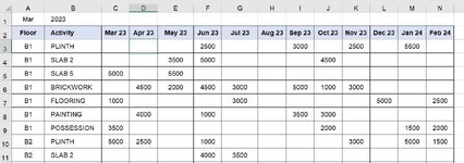
I have a Monthly Cashflow workbook with two worksheets viz. "Master" and "Cashflow". Master sheet has 7 Milestone Activities in the header B2:H2 and 5 Floor numbers in the first left column starting A3 : A12. (Each floor has 2 rows allotted, upper row shows the Month/year (mmm-yy) in which that amount will be received and the lower row shows the actual amount to be received.

MASTER.JPG


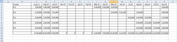
Second sheet "Cashflow" has floor numbers in column B (B2:B10) and Months (mmm-yy) in top header row C1:R1.

CASHFLOW.JPG


Currently I have manually linked cells from "Master" to the respective Month/Floor Cell in Cashflow. I am trying to figure out a way to automate this process where depending on the Month entered for a specific floor and specific activity can displayed under that month in cashflow in the respective floor row. If it can also display the respective activity name for that value, it would be an added advantage.

I tried reading Index/ Match options, but I am getting confused with how to start as I have 3 parameters in the Master table i.e. Floor, Activity and Month and not sure how to translate that into the cashflow.

could anyone please help ? Thanks in advance
 

Attachments

  • CASHFLOW.JPG
    CASHFLOW.JPG
    104.7 KB · Views: 4

Excel Facts

Do you hate GETPIVOTDATA?
Prevent GETPIVOTDATA. Select inside a PivotTable. In the Analyze tab of the ribbon, open the dropown next to Options and turn it off
Have you an option to restructure these two sheets as the way that they are laid out does not lend itself to the easiest solution?

Where do you reference the Activity in the Cashflow worksheet?

Do you use the first of the month in the cells representing the month or is it text?
 
Upvote 0
Hello Herakles

I am open to restructure the sheet as long as it serves the purpose and is in a user-friendly format. Actually, since this is only sample data, it has limited columns and rows. In my actual sheet there are many more columns and rows.

The activity in the Cashflow shall be referenced to Master sheet. Master sheet is where I manually enter month in front of each activity/ floor alongwith its value and the expect it to be displayed in correlating column/row in Cashflow based on floor and month.

I am trying to use month name text. So hoping to match month name in Master sheet to match with Month name in the Cashflow sheet while selecting the column in Cashflow sheet.
 
Upvote 0
Can I suggest this.

That the Master sheet be long and thin with the following columns.

Date
Floor
Activity
Amount

As time goes on and more data is available all you have to do is add rows.
This sheet is just used to collect and store data.

You can even have a seperate sheet to actually enter this information, row by row, and press a button to add it to the Master sheet.

It does not matter what order the data is stored in this sheet.

The date can either be
1 The date that the expense occurs.
2. The 1st of the month in which the expense occurs.
3. The 1st of the month in which you want the expense to be reported.

It is important that dates are stored as dates and not text.

From this data, standard Excel functions can be used to summarise it.

Onto the cash flow sheet.

Instead of having a sheet that that goes off into the distance to the right with a new column being added for each month can I suggest that
the sheet contains a column for each month (12) and these months can change dependant on what period you want to look at. The figures in the column
are the calculated based upon the month that the column represents.

Look at the image attached. (Data is just sample data.)

When the month and year in cells A1 and B1 change the column headings to represent the 12 months starting in the month and year specified
change and the data beneath them recalculates.

It also incorporates the Activity as you wanted.

Other summary sheets can be put together for information purposes.

Did you want to display the opening and closing balance for each month?
 

Attachments

  • Cashflow.JPG
    Cashflow.JPG
    108.6 KB · Views: 2
Upvote 0
@vikrampnz
For the future I suggest that you investigate XL2BB for providing sample data to make it easier for helpers by not having to manually type out sample data to test with.

In any case, see if this smaller sample works for you as it should be easily expanded for your extra rows.

vikrampnz.xlsm
ABCDEFGH
1
2Act 1Act 2Act 3Act 4Act 5Act 6Act 7
3B-1Aug-23Sep-23Oct-23Mar-24Apr-24May-24Nov-24
45863547
5B-2Aug-23Sep-23Oct-23May-24Jun-24Aug-24Nov-24
66985231
7
8
Master


vikrampnz.xlsm
ABCDEFGHIJKLMNOPQR
1Aug-23Sep-23Oct-23Nov-23Dec-23Jan-24Feb-24Mar-24Apr-24May-24Jun-24Jul-24Aug-24Sep-24Oct-24Nov-24
2B-15860000354000007
3
4B-26980000005203001
Cashflow
Cell Formulas
RangeFormula
C2:R2,C4:R4C2=SUMIF(INDEX(Master!$B$3:$H$6,MATCH($B2,Master!$A$3:$A$6,0),0),C$1,INDEX(Master!$B$3:$H$6,MATCH($B2,Master!$A$3:$A$6,0)+1,0))
 
Upvote 0
Hello Peter_SSs, your solution worked brilliantly. Thank you so much for your help.
Herakles, thanks for your time too !
 
Upvote 0
You're welcome. Thanks for the follow-up. :)
 
Upvote 0

Forum statistics

Threads
1,215,071
Messages
6,122,964
Members
449,094
Latest member
Anshu121

We've detected that you are using an adblocker.

We have a great community of people providing Excel help here, but the hosting costs are enormous. You can help keep this site running by allowing ads on MrExcel.com.
Allow Ads at MrExcel

Which adblocker are you using?

Disable AdBlock

Follow these easy steps to disable AdBlock

1)Click on the icon in the browser’s toolbar.
2)Click on the icon in the browser’s toolbar.
2)Click on the "Pause on this site" option.
Go back

Disable AdBlock Plus

Follow these easy steps to disable AdBlock Plus

1)Click on the icon in the browser’s toolbar.
2)Click on the toggle to disable it for "mrexcel.com".
Go back

Disable uBlock Origin

Follow these easy steps to disable uBlock Origin

1)Click on the icon in the browser’s toolbar.
2)Click on the "Power" button.
3)Click on the "Refresh" button.
Go back

Disable uBlock

Follow these easy steps to disable uBlock

1)Click on the icon in the browser’s toolbar.
2)Click on the "Power" button.
3)Click on the "Refresh" button.
Go back
Back
Top