WilliamPorter
New Member
- Joined
- Aug 5, 2021
- Messages
- 2
- Office Version
- 365
- Platform
- MacOS
Hello Excel Gurus!
I have a table that I'm trying to build. I have seen what I'm trying to do be done in an excel sheet but can not find a reference of it being done within a table.
I am running into the issue that when a number is divided out it is not equal so the pennies need to be added to variable cells.
I've used this posthttps://www.mrexcel.com/board/threads/dividing-a-number-and-returning-variable-results.485265/ and can get it to work on a sheet with set cells.
I need something this is dynamic, that I can use as a template, doesn't matter if it has 5 or 500 rows.
Can someone please help me develop a formula or give me some insight?
Thanks for your time.

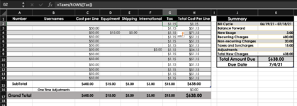
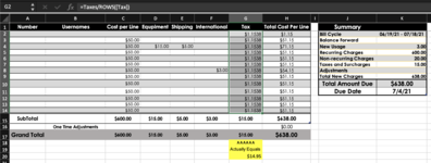
This happens because of how the taxes are not an even spread.

So i took the range and added a round down function so that would not happen

I'd like to be able to add the remaining $0.05 to varaible cells.

I have a table that I'm trying to build. I have seen what I'm trying to do be done in an excel sheet but can not find a reference of it being done within a table.
I am running into the issue that when a number is divided out it is not equal so the pennies need to be added to variable cells.
I've used this posthttps://www.mrexcel.com/board/threads/dividing-a-number-and-returning-variable-results.485265/ and can get it to work on a sheet with set cells.
I need something this is dynamic, that I can use as a template, doesn't matter if it has 5 or 500 rows.
Can someone please help me develop a formula or give me some insight?
Thanks for your time.
This happens because of how the taxes are not an even spread.
So i took the range and added a round down function so that would not happen
I'd like to be able to add the remaining $0.05 to varaible cells.
| New Billing SS Proposal - Example - WP.xlsx | |||||||||||||
|---|---|---|---|---|---|---|---|---|---|---|---|---|---|
| A | B | C | D | E | F | G | H | I | J | K | |||
| 1 | Number | Usernames | Cost per Line | Equpiment | Shipping | International | Tax | Total Cost Per Line | Summary | ||||
| 2 | xxxxxx | xyz | $1.15 | $1.15 | Bill Cycle | 06/19/21 - 07/18/21 | |||||||
| 3 | xxxxxx | xyz | $50.00 | $1.15 | $51.15 | Balance Forward | |||||||
| 4 | xxxxxx | xyz | $50.00 | $15.00 | $5.00 | $1.15 | $71.15 | New Usage | 3.00 | ||||
| 5 | xxxxxx | xyz | $50.00 | $1.15 | $51.15 | Recurring Charges | 600.00 | ||||||
| 6 | xxxxxx | xyz | $50.00 | $1.15 | $51.15 | Non-recurring Charges | 20.00 | ||||||
| 7 | xxxxxx | xyz | $50.00 | $1.15 | $51.15 | Taxes and Surcharges | 15.00 | ||||||
| 8 | xxxxxx | xyz | $50.00 | $3.00 | $1.15 | $54.15 | Adjustments | ||||||
| 9 | xxxxxx | xyz | $50.00 | $1.15 | $51.15 | Total New Charges | 638.00 | ||||||
| 10 | xxxxxx | xyz | $50.00 | $1.16 | $51.16 | Total Amount Due | $638.00 | ||||||
| 11 | xxxxxx | xyz | $50.00 | $1.16 | $51.16 | Due Date | 7/4/21 | ||||||
| 12 | xxxxxx | xyz | $50.00 | $1.16 | $51.16 | ||||||||
| 13 | xxxxxx | xyz | $50.00 | $1.16 | $51.16 | ||||||||
| 14 | xxxxxx | xyz | $50.00 | $1.16 | $51.16 | ||||||||
| 15 | SubTotal | $600.00 | $15.00 | $5.00 | $3.00 | $15.00 | $638.00 | ||||||
| 16 | One Time Adjustments | $0.00 | |||||||||||
| 17 | Grand Total | $600.00 | $15.00 | $5.00 | $3.00 | $15.00 | $638.00 | ||||||
Master | |||||||||||||
| Cell Formulas | ||
|---|---|---|
| Range | Formula | |
| G2:G9 | G2 | =ROUNDDOWN(Taxes/ROWS([Tax]),2) |
| C15 | C15 | =SUBTOTAL(109,[Cost per Line]) |
| D15 | D15 | =SUBTOTAL(109,[Equpiment]) |
| E15 | E15 | =SUBTOTAL(109,[Shipping]) |
| F15 | F15 | =SUBTOTAL(109,[International]) |
| G15 | G15 | =SUBTOTAL(109,[Tax]) |
| H2:H14 | H2 | =SUM(Bill9[@[Cost per Line]:[Tax]]) |
| H15 | H15 | =SUBTOTAL(109,[Total Cost Per Line]) |
| H16 | H16 | =SUM(C16:G16) |
| C17 | C17 | =Bill9[[#Totals],[Cost per Line]] |
| D17 | D17 | =Bill9[[#Totals],[Equpiment]] |
| E17 | E17 | =Bill9[[#Totals],[Shipping]] |
| F17 | F17 | =Bill9[[#Totals],[International]] |
| G17 | G17 | =Bill9[[#Totals],[Tax]] |
| H17 | H17 | =SUM(Bill9[[#Totals],[Total Cost Per Line]]+H16) |
| Named Ranges | ||
|---|---|---|
| Name | Refers To | Cells |
| Taxes | =Master!$K$7 | G2:G9 |