Dynamic average_range by column text in AVERAGEIFS formula

[g3lo18]

Hi,

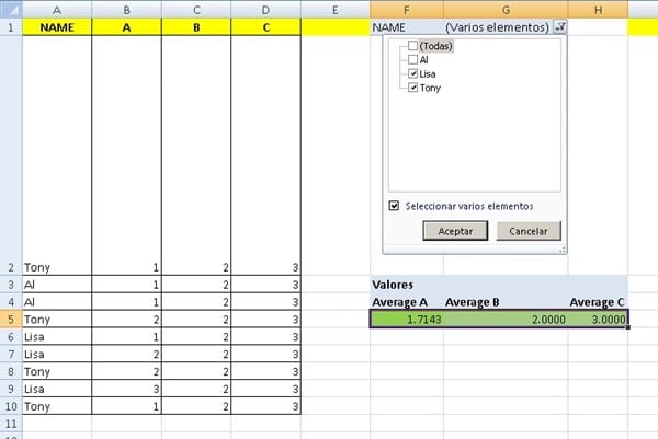
I am trying to obtain an average from multiple criteria using AVERAGEIFS function. The issue is I want to be able to specify the average range in a dynamic way based on column header name. I used index/match to specify the column name using header name for AVERAGEIF and it works like a charm. However, when using the same method in AVERAGEIFS it produces a #VALUE ! error. A simple example is attached. Please note there are two worksheets. Kindly advise if you have any solution to what I am trying to accomplish.

Many thanks!
g3lo18

worksheet "data example":

	A	B	C
Tony	1	2	3
Al	1	2	3
Al	1	2	3
Tony	1	2	3
Lisa	1	2	3
Lisa	1	2	3
Tony	1	2	3
Lisa	1	2	3
Tony	1	2	3

<tbody>
</tbody>

Main "Sheet2":

	AVERAGEIF works		AVERAGEIFS does not
	Tony		Tony + Lisa
A	1	=AVERAGEIF('data example'!A:A,"Tony",INDEX('data example'!$A$1:$D$10,0,MATCH(Sheet2!$A3,'data example'!$A$1:$D$1,0)))	#VALUE !	=AVERAGEIFS(INDEX('data example'!$A$1:$D$10,0,MATCH(Sheet2!$A3,'data example'!$A$1:$D$1,0)),'data example'!A:A,"Tony",'data example'!A:A,"Lisa")
B	2	=AVERAGEIF('data example'!A:A,"Tony",INDEX('data example'!$A$1:$D$10,0,MATCH(Sheet2!$A4,'data example'!$A$1:$D$1,0)))	#VALUE !	=AVERAGEIFS(INDEX('data example'!$A$1:$D$10,0,MATCH(Sheet2!$A4,'data example'!$A$1:$D$1,0)),'data example'!A:A,"Tony",'data example'!A:A,"Lisa")
C	3	=AVERAGEIF('data example'!A:A,Sheet2!$B$2,INDEX('data example'!$A$1:$D$10,0,MATCH(Sheet2!$A5,'data example'!$A$1:$D$1,0)))	#VALUE !	=AVERAGEIFS(INDEX('data example'!$A$1:$D$10,0,MATCH(Sheet2!$A5,'data example'!$A$1:$D$1,0)),'data example'!A:A,"Tony",'data example'!A:A,"Lisa")

<tbody>
</tbody>

Thank you!

 

[g3lo18]

I need to be able to average "is not" on multiple criteria as the sample data I provided you with is simplified. The actual data has over 200 unique variables, and if I name each one, it will take forever. I need to be able to say average 198 variables and avoid 2 ofthem. Or, average 197 variables, and avoid 3 of them, etc.

If it is Tony it cant also be Lisa nor can it be Frank. Give examples of cell values and whether you want them counted in the average or not.

 

[g3lo18]

I tried this, and this does not work with <> functions. Here is what I did:

=SUMPRODUCT(((A2:A10<>"*Tony*")+(A2:A10<>"Lisa"))*(B1:D1=F2)*(B2:D10))/SUMPRODUCT(((A2:A10<>"*Tony*")+(A2:A10<>"Lisa"))+0)

Provides the wrong average. I checked manually to see if it works.

Try this:

data example

	A	B	C	D	E	F	G
1		A	B	C			AVERAGEIF
2	Tony	1	2	3		A
3	Al	1	2	3		Tony
4	Al	1	2	3		Lisa	1.7142857
5	Tony	2	2	3
6	Lisa	1	2	3
7	Lisa	2	2	3
8	Tony	2	2	3
9	Lisa	3	2	3
10	Tony	1	2	3

<tbody>
</tbody>

Cell Formula G4 =SUMPRODUCT(((A2:A10=F3)+(A2:A10=F4))*(B1:D1=F2)*(B2:D10))/SUMPRODUCT(((A2:A10=F3)+(A2:A10=F4))+0) <tbody> </tbody>

<tbody>
</tbody>

 

[steve the fish]

This will do the average where the cell contains neither Lisa nor Tony

=AVERAGE(IF((NOT(ISNUMBER(SEARCH("Lisa",$A$2:$A$10))))*(NOT(ISNUMBER(SEARCH("Tony",$A$2:$A$10)))),INDEX('data example'!$A$2:$D$10,0,MATCH(Sheet2!$A3,'data example'!$A$1:$D$1,0))))

 

[g3lo18]

Thanks for the continue guidance. I tried this, when I don't click ctrl+shift+enter it works but displays the same number irrelevant of which column name you use. If I do an array (cntrl+shift+enter) it shows #N/A. :S

This will do the average where the cell contains neither Lisa nor Tony

=AVERAGE(IF((NOT(ISNUMBER(SEARCH("Lisa",$A$2:$A$10))))*(NOT(ISNUMBER(SEARCH("Tony",$A$2:$A$10)))),INDEX('data example'!$A$2:$D$10,0,MATCH(Sheet2!$A3,'data example'!$A$1:$D$1,0))))

 

[DanteAmor]

Another option is to create a pivot table, in it you can filter by one several items and get the average of A, B and C at the same time

 

[DanteAmor]

I tried this, and this does not work with <> functions. Here is what I did:

=SUMPRODUCT(((A2:A10<>"*Tony*")+(A2:A10<>"Lisa"))*(B1:D1=F2)*(B2:D10))/SUMPRODUCT(((A2:A10<>"*Tony*")+(A2:A10<>"Lisa"))+0)

Provides the wrong average. I checked manually to see if it works.

For that you need another type of formula, your requirement is to average Tony and Lisa. Not any combination.

 

[g3lo18]

I think it worked, I had one issue there I made. Thanks so much!

This will do the average where the cell contains neither Lisa nor Tony

=AVERAGE(IF((NOT(ISNUMBER(SEARCH("Lisa",$A$2:$A$10))))*(NOT(ISNUMBER(SEARCH("Tony",$A$2:$A$10)))),INDEX('data example'!$A$2:$D$10,0,MATCH(Sheet2!$A3,'data example'!$A$1:$D$1,0))))

 

[g3lo18]

Thanks for the alternative suggestion!

For that you need another type of formula, your requirement is to average Tony and Lisa. Not any combination.

 

[g3lo18]

I run into a problem using this formula counting blanks. Is there a way to ensure this formula does not account for blanks?

This will do the average where the cell contains neither Lisa nor Tony

=AVERAGE(IF((NOT(ISNUMBER(SEARCH("Lisa",$A$2:$A$10))))*(NOT(ISNUMBER(SEARCH("Tony",$A$2:$A$10)))),INDEX('data example'!$A$2:$D$10,0,MATCH(Sheet2!$A3,'data example'!$A$1:$D$1,0))))

 

[steve the fish]

=AVERAGE(IF(($A$2:$A$10<>"")*(NOT(ISNUMBER(SEARCH("Lisa",$A$2:$A$10))))*(NOT(ISNUMBER(SEARCH("Tony",$A$2:$A$10)))),INDEX('data example'!$A$2:$D$10,0,MATCH(Sheet2!$A3,'data example'!$A$1:$D$1,0))))