Dynamic chart based on month

[Plexzuz]

Hello! My firts post here! My English isnt great, but i will try anyway!

What i need is a dynamic chart that change the value on the chart based on a drop down list.
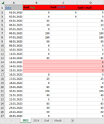
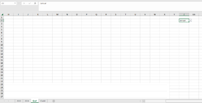
All the data i have is in sheet 1 named "2023". the other other sheet where i have all the charts is in sheet 2 "Graf".
In sheet 1(2023) the date is sorted from A2->A366 In the format 01.01.2023->31.12.2023.
the data is also in sheet 1 D2->D366.

I want a drop down list in sheet 2(graf) at Z2 to choose from January->Desember (I got it in norwegian btw. Dont know if that has anything to say) and pick up the date and data from sheet 1 for the month January->Desember. so when i choose January it will change the chart on sheet 2 and update the data there based on the month in the dropdown list.

How can i do this?

 

[Plexzuz]

Bump

 

[skillilea]

Filter is a newer dynamic function. This is probably a good place to start.

Here is a good overview:

 

[Plexzuz]

I have tried. But i can't get it to work

 

[skillilea]

I'll look at it in a bit. Give me a couple hours.

 

[skillilea]

Here is a sample data table. Its name is tblData

Date	Data
1/1/2023	10
1/2/2023	15
1/3/2023	20
1/4/2023	25
1/5/2023	30
1/6/2023	35
1/7/2023	40
1/8/2023	45
1/9/2023	50
1/10/2023	55
1/11/2023	60
1/12/2023	65
1/13/2023	70
1/14/2023	75
1/15/2023	80
1/16/2023	85
1/17/2023	90
1/18/2023	95
1/19/2023	100
1/20/2023	105
1/21/2023	110
1/22/2023	115
1/23/2023	120
1/24/2023	125
1/25/2023	130
1/26/2023	135
1/27/2023	140
1/28/2023	145
1/29/2023	150
1/30/2023	155
1/31/2023	160
2/1/2023	165
2/2/2023	170
2/3/2023	175
2/4/2023	180
2/5/2023	185
2/6/2023	190
2/7/2023	195
2/8/2023	200
2/9/2023	205
2/10/2023	210
2/11/2023	215
2/12/2023	220
2/13/2023	225
2/14/2023	230
2/15/2023	235
2/16/2023	240
2/17/2023	245
2/18/2023	250

 

[skillilea]

Now on your graf page.

1. Put a drop down list with your dates. Mine are 1/1/2023, 2/1/2023
the cell is in C2

2. Put this formula where you want the chart data
=FILTER(tblData, MONTH(tblData[Date]) = MONTH(C2), "")

3. Now highlight the data and add your chart.

I'll post a sample in second

 

[skillilea]

Book1
	B	C	D	E	F	G	H	I	J	K	L	M	N	O	P		R
1					Chart Data
2	Filter	1/1/2023			1/1/2023	10
3					1/2/2023	15
4					1/3/2023	20
5					1/4/2023	25
6					1/5/2023	30
7					1/6/2023	35
8					1/7/2023	40
9					1/8/2023	45
10					1/9/2023	50
11					1/10/2023	55
12					1/11/2023	60
13					1/12/2023	65
14					1/13/2023	70
15					1/14/2023	75
16					1/15/2023	80
17					1/16/2023	85
18					1/17/2023	90
19					1/18/2023	95
20					1/19/2023	100
21					1/20/2023	105
22					1/21/2023	110
23					1/22/2023	115
24					1/23/2023	120
25					1/24/2023	125
26					1/25/2023	130
27					1/26/2023	135
28					1/27/2023	140
29					1/28/2023	145
30					1/29/2023	150
31					1/30/2023	155
32					1/31/2023	160
Graf

Cell Formulas
Range	Formula
F2:G32	F2	=FILTER(tblData, MONTH(tblData[Date]) = MONTH(C2), "")
Dynamic array formulas.

Cells with Data Validation
Cell	Allow	Criteria
C2	List	=$Q$2:$Q$3