Dynamic chart range based on 2 values

[Lilium]

Hi,

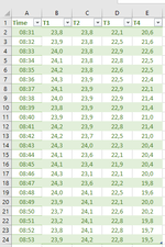
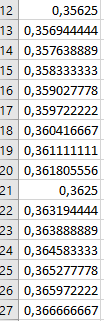
I have a table in a "Data" sheet with temperature readings from 4 locations (Columns B to E for locations T1, T2, T3 and T4) and different temperature readings (B2:E24) in those locations on different timeframes (A2:A24).
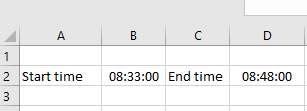
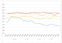
Now I have a sheet "Graphs" with a line chart of the temperature readings on those 4 locations, but I would like the graph to show only the readings based on the timeframe selected on sheet "Analysis" from cell B2 (start time) and cell D2 (End time).

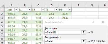
How do I do this? I tried making a name for the temperature range and adding this formula for the name: INDEX(Data!A$2:E$24;MATCH(Analysis!$B$2;Data!$A$2:$A$24;1)):INDEX(Data!A$2:E$24;MATCH(Analysis!$D$2;Data!$A$2:$A$24;1))
and another name for the timeframe and adding this formula:
INDEX(Data!A$2:A$24;MATCH(Analysis!$B$2;Data!$A$2:$A$24;1)):INDEX(Data!A$2:A$24;MATCH(Analysis!$D$2;Data!$A$2:$A$24;1))
and then putting this in the data range of the graph but I don't get it to work.

What am I doing wrong?

Thanks

 

[levipe]

It would be helpful to know how it doesn't work but at first glance, your temperature formula appears to have a typo. You have

INDEX(Data![B]A$2[/B]:E$24;MATCH(Analysis!$B$2;Data!$A$2:$A$24;1)):INDEX(Data!A$2:E$24;MATCH(Analysis!$D$2;Data!$A$2:$A$24;1))

Seems like it should be

INDEX(Data![B]E$2[/B]:E$24;MATCH(Analysis!$B$2;Data!$A$2:$A$24;1)):INDEX(Data!A$2:E$24;MATCH(Analysis!$D$2;Data!$A$2:$A$24;1))

I suggest putting the formula into a cell (select several rows) and confirm as an array formula with Ctrl+Shift+Enter and it'll show you the output.

 

[Fluff]

@levipe if you are going to format something inside tags, you need to use the RICH tags.

 

[Lilium]

Thank you levipe. I've pasted the formula in the cels and i get output now: see attached screenshot.
But then how do I incorporate this in my data range selection of my graph? I just can't figure it out. (see screenshot)

 

[levipe]

If the output you're getting from the formula in the worksheet is what you want, then go back to your original plan and put that formula into a name. The idea of putting the formula into a cell is just so we could see what the output was and why it wasn't working.