Dynamic Power Query (web)

[Abdmujib]

I want to use power query to extract a table from the web.

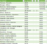
In the picture below, I loaded a table from this website Premier League Form Table
there are multiple websites that has the same table structure and with the same table position, that I will love to switch to without having to go to power query, maybe by pasting the website in the cell B2 and then the table for the particular link load.

so, I paste the link for spain in Cell B2 , the table loads for , spain without having to go to power query to put spain link into it.

pls kindly help. thanks

 

[Abdmujib]

I duplicated the sheet named "DATA" and I switched the country from the dropdown button and refreshed in order to load for the choosen country but, it didn't effect the changes.

I have gotten a way round it. I renamed the "SelectedCountry" into another name. I also replace the "SelectedCountry" in the source code to the new name.

Thank you so much. But it would have been easy if the name in the source code can fetch the sheet name and the reference of the cell, i.e Sheet1!A9, if another sheet is duplicated, that it will fetch the record in Sheet2!A9 and so on an so forth. It will be more dynamic that way.

 

[Alex Blakenburg]

I don't believe you can get a single query to output to multiple tables. I think that you would need to use VBA do what you are asking.

 

[Abdmujib]

I don't believe you can get a single query to output to multiple tables. I think that you would need to use VBA do what you are asking.

Oh okay, I believe that's one of the few advantages of Google sheet over excel. I prefer renaming the cell from "selectedcountry" over vba code. It's always difficult for me to maintain when the website changes their structural framework.

 

[Abdmujib]

@Alex

 

[Abdmujib]

I don't believe you can get a single query to output to multiple tables. I think that you would need to use VBA do what you are asking.

Hello Good morning, Pls can you help me to do another similar workbook, I have been trying to replicate it through the one you sent me through your deive but the contents of the tablle are different so it makes it difficult for me.

Thanks

 

[Abdmujib]

Hello @Alex Blakenburg,

pls can you help me to reproduce the dynamic power query for another workbook. I tried to reproduce it using the one you gave me the last time but I could not get it.

in this workbook. what I want to do is in sheet "Basketball" , In the Sheet B2 and C2 are Data validation columns, which the country is selected from the the data validation and also C2 is where the league would be chosen. When that is done, the link for the fixtures would pop out in D2 while the link of the result table will pop out at E2 for the specific League that was chosen.

Note:
D2 has been name tagged "Fixture1" while E2 named "RLink1"

Results

I want the past matches Results query data to load cell BC5. it's link would be in cell E2 (RLink1). Please do not remove any of its column.

Fixtures

I want the past fixtures query data to load cell A335. it's link would be in cell D2 (Fixture1). Please do not remove any of its column. if possible help me to limit the fixtures to 55 rows only. thanks

The Workbook

 

[Alex Blakenburg]

Start with this for the results part (RLink1 > BC5).
It is almost straight off the link below:

1. Create a new Blank Query and copy in the first lot of code below and call the query >
   functionGetNamedRange
2. Create a second blank query and copy in the 2nd lot of code below, give it a meaningful name and then close and load it with a destination of BC5
3. See how the results look and come back to me on what works and what doesn't and what we need to change.

1) functionGetNamedRange

let GetNamedRange=(NamedRange) =>
 
let
    name = Excel.CurrentWorkbook(){[Name=NamedRange]}[Content],
    value = name{0}[Column1]
in
    value

in GetNamedRange

2) Report

let
    Source = Web.Page(Web.Contents(functionGetNamedRange("RLink1"))),
    Data0 = Source{0}[Data],
    #"Changed Type" = Table.TransformColumnTypes(Data0,{{"Semi-finals - 3rd leg", type text}, {"Semi-finals - 3rd leg2", type text}, {"1", Int64.Type}, {"2", Int64.Type}, {"", type date}})
in
    #"Changed Type"

Link

How To Reference A Named Range In Power Query | How To Excel

www.howtoexcel.org

 

[Abdmujib]

Than

Start with this for the results part (RLink1 > BC5).
It is almost straight off the link below:

1. Create a new Blank Query and copy in the first lot of code below and call the query >
   functionGetNamedRange
2. Create a second blank query and copy in the 2nd lot of code below, give it a meaningful name and then close and load it with a destination of BC5
3. See how the results look and come back to me on what works and what doesn't and what we need to change.

1) functionGetNamedRange

let GetNamedRange=(NamedRange) =>
 
let
    name = Excel.CurrentWorkbook(){[Name=NamedRange]}[Content],
    value = name{0}[Column1]
in
    value

in GetNamedRange

2) Report

let
    Source = Web.Page(Web.Contents(functionGetNamedRange("RLink1"))),
    Data0 = Source{0}[Data],
    #"Changed Type" = Table.TransformColumnTypes(Data0,{{"Semi-finals - 3rd leg", type text}, {"Semi-finals - 3rd leg2", type text}, {"1", Int64.Type}, {"2", Int64.Type}, {"", type date}})
in
    #"Changed Type"

Link

How To Reference A Named Range In Power Query | How To Excel

www.howtoexcel.org

Kbyou so much, I will try it out

 

[Abdmujib]

Start with this for the results part (RLink1 > BC5).
It is almost straight off the link below:

1. Create a new Blank Query and copy in the first lot of code below and call the query >
   functionGetNamedRange
2. Create a second blank query and copy in the 2nd lot of code below, give it a meaningful name and then close and load it with a destination of BC5
3. See how the results look and come back to me on what works and what doesn't and what we need to change.

1) functionGetNamedRange

let GetNamedRange=(NamedRange) =>
 
let
    name = Excel.CurrentWorkbook(){[Name=NamedRange]}[Content],
    value = name{0}[Column1]
in
    value

in GetNamedRange

2) Report

let
    Source = Web.Page(Web.Contents(functionGetNamedRange("RLink1"))),
    Data0 = Source{0}[Data],
    #"Changed Type" = Table.TransformColumnTypes(Data0,{{"Semi-finals - 3rd leg", type text}, {"Semi-finals - 3rd leg2", type text}, {"1", Int64.Type}, {"2", Int64.Type}, {"", type date}})
in
    #"Changed Type"

Link

How To Reference A Named Range In Power Query | How To Excel

www.howtoexcel.org

Hello, Pls I didn't get it, also there are two query which I want to load into the workbook Fixture1 an RLink1. the Rlink.

For the Country and league Pls Switch it to Spain and ACB. so it will be simpler. this is how I want the Rlink1 table to be (Picture attached named For PQ), which is to populate on BC5. the header do change week by week depending on the game round they are, even it can be different for another league, like it is semi final in Norway you did earlier.


The second table to be populated is Fixtures which has it link on D2 (Fixture1), the picture of how it will look like is attached. pls I want it populate on A335.

thank you sir.

I would be glad if you can help me do it on the workbook I sent to you sir

 

[Abdmujib]

Start with this for the results part (RLink1 > BC5).
It is almost straight off the link below:

1. Create a new Blank Query and copy in the first lot of code below and call the query >
   functionGetNamedRange
2. Create a second blank query and copy in the 2nd lot of code below, give it a meaningful name and then close and load it with a destination of BC5
3. See how the results look and come back to me on what works and what doesn't and what we need to change.

1) functionGetNamedRange

let GetNamedRange=(NamedRange) =>
 
let
    name = Excel.CurrentWorkbook(){[Name=NamedRange]}[Content],
    value = name{0}[Column1]
in
    value

in GetNamedRange

2) Report

let
    Source = Web.Page(Web.Contents(functionGetNamedRange("RLink1"))),
    Data0 = Source{0}[Data],
    #"Changed Type" = Table.TransformColumnTypes(Data0,{{"Semi-finals - 3rd leg", type text}, {"Semi-finals - 3rd leg2", type text}, {"1", Int64.Type}, {"2", Int64.Type}, {"", type date}})
in
    #"Changed Type"

Link

How To Reference A Named Range In Power Query | How To Excel

www.howtoexcel.org

it says "Expression.Error: The import functionGetNamedRange matches no exports. Did you miss a module reference?"