Dynamic Range

[bobkap]

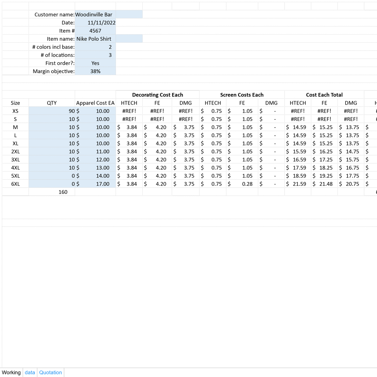
I have 2 named ranges - bk and bkt - that I wanted to make dynamic. I thought I correctly created them but when I did everything went haywire. Link to the file is below.

As you will see, it seemed to compute everything correctly except in cells D14,15; E14, 15; F14, F15. I just cannot seem to figure out why it will work in some cells but not others.

Any much needed help would be greatly appreciated.

Decorator price model v8.xlsm

Shared with Dropbox

www.dropbox.com

 

[jasonb75]

What should each one refer to if they were not dynamic? (based on the current data).

bk definitely contains an error, bkt looks ok but may not be depending on requirements.

 

[bobkap]

Thanks for asking! Disregarding being a dynamic range, I'd just like my "data" sheet data to all be in one named range.

Really appreciate the help! Curious as to what the error is in bk.

 

[jasonb75]

Curious as to what the error is in bk.

You had COUNTA(A1048575) instead of COUNTA(A:A) so it was trying to count a single empty cell at the bottom of the sheet instead of the actual data.

If yo want to make the data table truly dynamic (without making it volatile by using OFFSET) then I would go with the following method.

LastCol =MATCH(1e+100,Data!$1:$1)
LastRow =MATCH("zzz",Data!$A:$A)
bkt =Data!$B$1:INDEX(Data!$1:$1,LastCol)
bks =Data!$A$2:INDEX(Data!$A:$A,LastRow)
bk =Data!$B$2:INDEX(Data!$B:$B,LastRow):INDEX(Data!$2:$2,LastCol)

Using those definitions, bkt will give you the data in Row 1, bks will give you the data in Column A, bk will give you the rest of the table (excluding row 1 and column A).

Note that there is some clutter in column A starting from A36, it would be best to move this in order to make the dynamic ranges work properly. Dragging them to the right a bit will be fine, as long as there is no clutter in column A or row 1 it will work correctly.

 

[bobkap]

Mega thanks again!!! I love your solution of using several names too.

 

[bobkap]

You had COUNTA(A1048575) instead of COUNTA(A:A) so it was trying to count a single empty cell at the bottom of the sheet instead of the actual data.

If yo want to make the data table truly dynamic (without making it volatile by using OFFSET) then I would go with the following method.

LastCol =MATCH(1e+100,Data!$1:$1)
LastRow =MATCH("zzz",Data!$A:$A)
bkt =Data!$B$1:INDEX(Data!$1:$1,LastCol)
bks =Data!$A$2:INDEX(Data!$A:$A,LastRow)
bk =Data!$B$2:INDEX(Data!$B:$B,LastRow):INDEX(Data!$2:$2,LastCol)

Using those definitions, bkt will give you the data in Row 1, bks will give you the data in Column A, bk will give you the rest of the table (excluding row 1 and column A).

Note that there is some clutter in column A starting from A36, it would be best to move this in order to make the dynamic ranges work properly. Dragging them to the right a bit will be fine, as long as there is no clutter in column A or row 1 it will work correctly.

I don't mean to be a pest or appear ungrateful, but would you mind telling me what the "1e+100" does as well as the "zzz"? I can get the LastCol to work but the LastRow does not.

 

[jasonb75]

1E+100 finds the last numeric entry in a row / column.
"zzz" should find the last text entry (on the assumption that you don't have text entries that start with "zzz" in your actual data.

You do need to use the correct one for the type of data that you have, 1E+100 will not see any text in the row / column that it looks at, likewise "zzz" will not see numeric data.

There were also some odd entries lower down the sheet, the last row formula will still work with them there but will include them in the range along with any empty rows between them and the proper table.

 

[bobkap]

Thanks again. Now that I've named my ranges via defining the name process vs just highlighting and naming in that dropdown field just above the A1 cell, the names no longer appear in the drop down. Is there any way that I can see what cells my named range is covering now?

 

[jasonb75]

Possibly you're still using the old name?
You would need to use =bkt to return the numbers in row 1 to the dropdown and =bks to return the text in column A.

If you type bk, bkt, or bks into the that normally shows the address of the active cell (to the left of the formula bar) it should take you to that range and automatically select it.