Excel conditional formatting in a Gantt Chart

[mb8marmed]

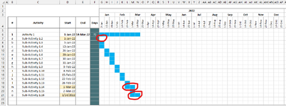
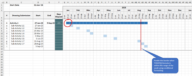
I was trying to provide conditional formatting in my Gantt Chart. However, I have difficulty developing a formula that will trigger to highlight the cell or range, as the date is not a usual one. I'm hoping that someone from this group can help me solve the issue. I manually provided the colors for visualization, and the conditional formatting is supposed to work on this, but it's not working the way I wanted.

Thank you in advance.

Gantt Chart Formula.xlsx
	B	C	D	E	F	G	H	I	J	K	L	M	N	O	P	Q	R	S	T	U	V	W	X	Y	Z	AA	AB	AC	AD	AE	AF	AG	AH	AI	AJ	AK	AL	AM	AN	AO	AP
1		Start Date	1-Jan-22
2						2022
3						Jan			Feb			Mar			Apr			May			Jun			Jul			Aug			Sep			Oct			Nov			Dec
4	#	Activity	Start	End	Days	2-Jan	15-Jan	28-Jan	1-Feb	14-Feb	27-Feb	1-Mar	14-Mar	27-Mar	1-Apr	14-Apr	27-Apr	1-May	14-May	27-May	1-Jun	14-Jun	27-Jun	1-Jul	14-Jul	27-Jul	1-Aug	14-Aug	27-Aug	1-Sep	14-Sep	27-Sep	1-Oct	14-Oct	27-Oct	1-Nov	14-Nov	27-Nov	1-Dec	14-Dec	27-Dec
5
6	1	Activity 1	2-Mar-22	21-Sep-22	203
7	a	Sub-Activity 1.2	2-Mar-22
8	b	Sub-Activity 1.3	5-Apr-22
9	c	Sub-Activity 1.4	15-May-22
10	d	Sub-Activity 1.5	30-Jun-22
11	e	Sub-Activity 1.6	8/10/2022
12	f	Sub-Activity 1.7	9/21/2022
13
14						1	2	3	1	2	3	1	2	3	1	2	3	1	2	3	1	2	3	1	2	3	1	2	3	1	2	3	1	2	3	1	2	3	1	2	3
Gantt Chart

Cell Formulas
Range	Formula
G1:M1,R1:AP1	G1	=IF(AND(MONTH(G$4)=MONTH($D6),AND($D6<=G$4*G$14*13,$D6<G$4)),"x","")
G2	G2	=T4
G3,J3,M3,P3,S3,V3,Y3,AB3,AE3,AH3,AK3,AN3	G3	=H4
G4	G4	=IF(MONTH(D1-WEEKDAY((D1),2)+1)<MONTH(D1),(D1-28-DAY(D1)+7)-WEEKDAY((D1-DAY(D1)+7),2)+1,(D1-DAY(D1)+7)-WEEKDAY((D1-DAY(D1)+7),2))
H4:AP4	H4	=IF(G4+13>EOMONTH(G4,0),EOMONTH(G4,0)+1,G4+13)
F5:F13	F5	=IF(AND(D5<>"",E5<>""),E5-D5,"")
G5:AP13	G5	=IF(AND(MONTH(G$4)=MONTH($D6),AND($D6<=G$4*G$14*13,$D6<G$4)),"x","")
D6	D6	=MIN(D7:D12)
E6	E6	=MAX(D7:D12)
Press CTRL+SHIFT+ENTER to enter array formulas.

 

[DanteAmor]

If you want 2 colors then you need 2 rules:

Dante Amor
	A	B	C	D	E	F	G	H	I	J	K	L	M	N	O	P	Q	R	S	T	U	V	W	X	Y	Z	AA	AB	AC	AD	AE	AF	AG	AH	AI	AJ	AK	AL	AM	AN	AO	AP
1			Start Date	01/01/2022
2							2022
3							Jan			Feb			Mar			Apr			May			Jun			Jul			Aug			Sep			Oct			Nov			Dec
4		#	Activity	Start	End	Days	02-ene	15-ene	28-ene	01-feb	14-feb	27-feb	01-mar	14-mar	27-mar	01-abr	14-abr	27-abr	01-may	14-may	27-may	01-jun	14-jun	27-jun	01-jul	14-jul	27-jul	01-ago	14-ago	27-ago	01-sep	14-sep	27-sep	01-oct	14-oct	27-oct	01-nov	14-nov	27-nov	01-dic	14-dic	27-dic
5
6		1	Activity 1	02-mar-22	21-sep-22	203
7		a	Sub-Activity 1.2	02-mar-22
8		b	Sub-Activity 1.3	05-abr-22
9		c	Sub-Activity 1.4	15-may-22
10		d	Sub-Activity 1.5	30-jun-22
11		e	Sub-Activity 1.6	10-ago-22
12		f	Sub-Activity 1.7	21-sep-22
Hoja1

Cells with Conditional Formatting
Cell	Condition		Cell Format	Stop If True
G6:AP12	Expression	=OR(AND(G$4>=$D6,G$4<=$E6),AND($D6>=G$4,$D6<=H$4,$E6<>""))	text	NO
G6:AP12	Expression	=OR(AND(G$4>=$D6,G$4<=$E6),AND($D6>=G$4,$D6<=H$4))	text	NO

 

[mb8marmed]

If you want 2 colors then you need 2 rules:

Dante Amor
	A	B	C	D	E	F	G	H	I	J	K	L	M	N	O	P	Q	R	S	T	U	V	W	X	Y	Z	AA	AB	AC	AD	AE	AF	AG	AH	AI	AJ	AK	AL	AM	AN	AO	AP
1			Start Date	01/01/2022
2							2022
3							Jan			Feb			Mar			Apr			May			Jun			Jul			Aug			Sep			Oct			Nov			Dec
4		#	Activity	Start	End	Days	02-ene	15-ene	28-ene	01-feb	14-feb	27-feb	01-mar	14-mar	27-mar	01-abr	14-abr	27-abr	01-may	14-may	27-may	01-jun	14-jun	27-jun	01-jul	14-jul	27-jul	01-ago	14-ago	27-ago	01-sep	14-sep	27-sep	01-oct	14-oct	27-oct	01-nov	14-nov	27-nov	01-dic	14-dic	27-dic
5
6		1	Activity 1	02-mar-22	21-sep-22	203
7		a	Sub-Activity 1.2	02-mar-22
8		b	Sub-Activity 1.3	05-abr-22
9		c	Sub-Activity 1.4	15-may-22
10		d	Sub-Activity 1.5	30-jun-22
11		e	Sub-Activity 1.6	10-ago-22
12		f	Sub-Activity 1.7	21-sep-22
Hoja1

Cells with Conditional Formatting
Cell	Condition		Cell Format	Stop If True
G6:AP12	Expression	=OR(AND(G$4>=$D6,G$4<=$E6),AND($D6>=G$4,$D6<=H$4,$E6<>""))	text	NO
G6:AP12	Expression	=OR(AND(G$4>=$D6,G$4<=$E6),AND($D6>=G$4,$D6<=H$4))	text	NO

Hi Mr. DanteAmor,

Thanks for the inputs, I tried your formula and expanded the chart, and it is almost there. However, at some point the formula "=OR(AND(G$4>=$D6,G$4<=$E6),AND($D6>=G$4,$D6<=H$4))", for the light blue color is not behaving properly for some dates such as:

01-Jan-2022
28-Jan-2022
01-Mar-2022
03-Mar-2022

Maybe you can help me on this. Thank you so much for the help.

mb8marmed

​

 

[DanteAmor]

"=OR(AND(G$4>=$D6,G$4<=$E6),AND($D6>=G$4,$D6<=H$4))"

Change that formula for this:

=OR(AND($D6>=G$4,$D6<H$4),AND($D6<$G$4,G$4=$G$4),$D6=G$4)

 

[mb8marmed]

Change that formula for this:

=OR(AND($D6>=G$4,$D6<H$4),AND($D6<$G$4,G$4=$G$4),$D6=G$4)

Hi DanteAmor,

The code is now working properly and speeds up my work significantly.

Thank you so much...

 

[mb8marmed]

Hi DanteAmor,

The code/formula for the light blue conditional formatting is working perfectly. Maybe you can help me to correct the formula for the dark blue conditional formatting.
=OR(AND(G$4>=$D5,G$4<=$E5),AND($D5>=G$4,$D5<=H$4,$E5<>""))

Additionally, if you can also provide a formula for the conditional formatting that will create border in the column once the TODAYS() date is within the range of the week as seen on the attachment.

Thank you and more power.

 

[DanteAmor]

=OR(AND(G$4>=$D5,G$4<=$E5),AND($D5>=G$4,$D5<=H$4,$E5<>""))

In your image there is no data in the cells of row 5, but in the formula that you put, you refer to cells of row 5

----- --

Maybe you can help me to correct the formula for the dark blue conditional formatting

I did other tests for the dark blue, try:

=OR(AND($E6<>"",G$4>=$D6,G$4<=$E6),AND($E6<>"",$D6>=G$4,$D6<H$4))

----- --

if you can also provide a formula for the conditional formatting that will create border in the column once the TODAYS() date is within the range of the week

Try:

=AND(TODAY()>=G$4,TODAY()<H$4)

 

[mb8marmed]

In your image there is no data in the cells of row 5, but in the formula that you put, you refer to cells of row 5

----- --


I did other tests for the dark blue, try:

=OR(AND($E6<>"",G$4>=$D6,G$4<=$E6),AND($E6<>"",$D6>=G$4,$D6<H$4))

----- --

Try:

=AND(TODAY()>=G$4,TODAY()<H$4)

Thank you so much for the help. It is now working well.