I'd like to temper your expectations regarding what can be achieved with an older version of Excel. Most of what you've described can be done in Excel 2007 using a formula-based approach, however, you'll see that many of the formulas are long, complex, and full of redundancy. Some of that could be mitigated by introducing additional helper cells to hold certain values that are used repeatedly. For now, I'm offering an approach that uses some helper cells for:
- storing the beginning and end of whichever month/year is specified in B1:B2;
- storing the beginning and end dates of the two vacation blocks, and
- storing the worksheet name, since you plan to use 1st, 2nd, and 3rd, this makes it convenient to use the sheet name to find which members are associated with those shift
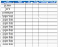
Before I describe the month output sheet, let's discuss the Master sheet. I recommend introducing an additional column so that the "Position" and the Member's name can be maintained separately. This makes it easier to determine the number of leaders, supervisors, etc. based on any of various functions that could simply utilize the terms found in the Position column. I also recommend making this Master table an official Excel table (I believe yours may be an official table, but I'm not certain). To convert a range to a table, click anywhere in the range, then Ctrl-t to pop open a small dialog box where you can confirm that the entire range to convert has been identified...and confirm that the table has headers. This conversion facilitates formula-writing and comprehension since structured references can be used (meaning we can refer to the table name and table headings rather than cell ranges). And if the table expands/contracts in size, the formulas relying on those ranges do not require editing. You didn't describe how the vacation block would be recorded...I've assumed it might have the format mm/dd/yyyy-mm/dd/yyyy to denote the start-end dates. As such, that text string needs to be split apart, and rather than do that with a fairly complex formula every time those dates are needed, the formulas appear in helper cells to the right of the month table (in columns AJ:AM) where those results can be referenced by other formulas.
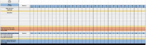
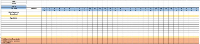
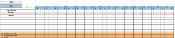
As for "auto fill"...user intervention is necessary with Excel 2007. This would not be the case with Excel 365, where the relevant members who are scheduled for the month would indeed "spill" down the worksheet based on the results of a single formula. But given these limitations of Excel 2007, the sample month sheet below for 1st Shift requires you to specify a year and month in B1:B2. The dates for that month and the day abbreviation are automatically created in rows 5:6. I suggest leaving the size of the "days" part of the table at 31 columns to accommodate any month (and blanks will simply be padded at the end for shorter months). Then the formula in A7 extracts the names of any "Members" who chose the shift matching the sheet name (1st, 2nd, or 3rd). This formula may not work well in Excel 2007...give it a try and let me know. Once entered, it it does not produce output, select the cell where the formula is found, hit F2 to enter "edit" mode, then reconfirm the formula by hitting Ctrl-Shift-Enter simultaneously to enter the formula as an array formula. You may need to then drag the formula to the right one column and down until no more results are produced. This manual intervention is necessary because Excel 2007 does not support "spilling" multiple results...you need to drag the formula until no more results appear. If the formula still gives you trouble, let me know...it may need to be split apart to return only one column at a time. I can't test it because I'm not using Excel 2007.
Then the day "field" of the month table uses a formula to determine...
- if that column heading date is not blank (if so, continue evaluating, otherwise a blank),
- if the date falls within the vacation block dates (if so, a "V"),
- if the day of the week coincides with that member's "weekend" days off (if so, an "X")
- and if neither of the two above, then a blank
You will need to drag this formula throughout the relevant month range to get it to populate with results.
You might consider moving the orange "Total" rows to a location above the month table. The rationale for this is that the upper part of your month worksheet would be relatively static, and as the month table grows in length, you won't need to shift the orange Total rows down (maybe this isn't a problem if you have a reasonable upper limit on the length of the month table and set the sheet up to reflect that potential growth). Finally, I'm not certain about which positions get counted as "Supervision" and "Classification Specialists"...I've set up the formulas to allow for multiple types of positions to be counted, but you may need to revise accordingly.
| MrExcel_20231122.xlsx |
|---|
|
|---|
| A | B | C | D | E | F |
|---|
| 1 | Position | Members | Shift | Days Off | 1st Approved Vacation | 2nd Approved Vacation |
|---|
| 2 | Shift Supervisors | foxtrot | 1st | MT | 3/7/2024-3/16/2024 | 4/2/2024-4/15/2024 |
|---|
| 3 | Shift Supervisors | delta | 3rd | | | |
|---|
| 4 | Shift Supervisors | lima | 2nd | | | |
|---|
| 5 | Shift Supervisors | mike | 1st | WT | 3/11/2024-3/16/2024 | |
|---|
| 6 | Team Leaders | charlie | 2nd | | | |
|---|
| 7 | Team Leaders | juliett | 1st | SS | 3/20/2024 | 4/7/2024 |
|---|
| 8 | Team Leaders | | | | | |
|---|
| 9 | Job Assignment | alpha | 2nd | | | |
|---|
| 10 | Job Assignment | kilo | 2nd | | | |
|---|
| 11 | Job Assignment | bravo | 1st | TW | | |
|---|
| 12 | Reclassification | india | 2nd | | | |
|---|
| 13 | Reclassification | echo | 1st | TF | 3/3/2024-3/6/2024 | 3/27/2024-3/30/2024 |
|---|
| 14 | Reclassification | | | | | |
|---|
| 15 | Specialists | golf | 3rd | | | |
|---|
| 16 | Specialists | hotel | 1st | FS | | |
|---|
| 17 | | | | | | |
|---|
|
|---|
These formulas are dragged out to column AG so that there are 31 columns to accommodate any month:
And the helper cells to the right of the month table (be sure to select all four vacation start/end formulas and drag the formulas down so that they can "operate" on any members added to the month table):