EXCEL QUARY

[TANUSREE]

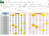
THERE IS TWO TABLE..''NUMBER TABLE & LAST DRAWN " .

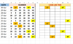
IN NUMBER TABLE I HIGHLIGHTED A NUMER " 17 " WHICH YOU SEE APPEARS ON 30th, 24th, 23rd & 19th April respectively.

IN THE "LAST DRAWN " TABLE, I HAVE PICKED THE NUMBER 17 THAT APPEARS 6 FROM THE TABLE ( 30TH - 24TH APRIL) AND HIGHLIGHTED IT TO SHOW IT APPEARED 6 DAYS EARLIER ( HIGHLIGHTED IN YELLOW) THEN I HIGHLIGHTED THE NEXT NUMBER 1 ( 24TH-23RD) APRIL. & SO ON...

The attached xls sheet is an illustration, is there a formula so that whenever I write down the number 17 .... it automatically shows the last drawn number like 6 , 4 , 1 in the chart....
Looking forward to hearing from you ,

 

[KRice]

Give this a try:

MrExcel_20220426.xlsm
	A	B	C	D	E	F	G	H	I	J	K	L	M	N
1	Date	Numbers							Last Drawn
2	4/30/2022	28	7	48	25	18	35		6	7	3	16	9	4
3	4/29/2022	10	46	44	34	3	24		6	8	13	1	17	4
4	4/28/2022	8	47	34	31	14	30		14	10	11	3	12	13
5	4/27/2022	29	15	39	48	42	12		5	11	9	none	13	2
6	4/26/2022	35	9	32	6	16	13		1	1	2	6	11	6
7	4/25/2022	9	12	24	35	23	31		5	1	2	3	8	4
8	4/24/2022	49	12	32	33	28	40		3	none	4	12	7	5
9	4/23/2022	22	19	10	24	7	11		5	1	none	none	1	none
10	4/22/2022	27	29	19	35	7	45		5	none	none	7	4	3
11	4/21/2022	41	18	26	49	46	31		2	2	none	none	9	6
12	4/20/2022	6	21	9	2	13	32		none	1	4	none	none	9
13	4/19/2022	4	40	21	41	18	45		2	3	5	6	3	1
14	4/18/2022	17	39	45	7	47	22		5	7	none	3	none	7
15	4/17/2022	34	28	23	38	4	27		none	none	none	3	4	none
16	4/16/2022	18	9	40	14	44	15		1	4	3	4	2	6
17	4/15/2022	18	16	7	31	30	35		none	5	none	5	none	2
18	4/14/2022	42	38	44	21	8	25		none	none	3	none	1	none
19	4/13/2022	35	4	17	41	40	8		none	none	none	none	1	none
20	4/12/2022	40	9	46	33	14	3		none	none	1	none	none	1
21	4/11/2022	3	22	32	44	46	39		none	none	1	none	none	none
22	4/10/2022	31	16	20	43	32	15		0	0	0	0	0	0
Sheet10

Cell Formulas
Range	Formula
I2:N21	I2	=IFERROR(AGGREGATE(15,6,(ROW($A3:$A$22)-ROW($A2))/--($B3:$G$22=B2),1),"none")
I22:N22	I22	=IFERROR(AGGREGATE(15,6,(ROW($A$22:$A23)-ROW($A22))/--($B$22:$G23=B22),1),"none")

 

[TANUSREE]

IS THERE ANY FORMULA TO DELETE THE NUMBER WITHOUT DELETING ROW & COLUMN..? ( in my attachment i need only 17 & 47 so in "look like table " i deleted all other numbers manually except 17 & 47 )

PLEASE FIND THE ATTACHMENT BELOW..

 

[KRice]

What rule applies to say that you need only 17 and 47? For example, why not show 26 and 30, and no other numbers? The answers to those questions affect the approach to your question.

 

[KRice]

One idea is to rebuild your initial table and specify which number you want to see, and insert blanks anywhere else, and then use conditional formatting to color the cells of each selected number.

MrExcel_20220426.xlsm
	A	B	C	D	E	F	G	H	I	J	K	L	M	N	O	P	Q	R	S	T	U
1																Show only		28	48	35
2	Date	Numbers							Last Drawn							Selected Numbers
3	4/30/2022	28	7	48	25	18	35		6	7	3	16	9	4		28		48			35
4	4/29/2022	10	46	44	34	3	24		6	8	13	1	17	4
5	4/28/2022	8	47	34	31	14	30		14	10	11	3	12	13
6	4/27/2022	29	15	39	48	42	12		5	11	9	none	13	2					48
7	4/26/2022	35	9	32	6	16	13		1	1	2	6	11	6		35
8	4/25/2022	9	12	24	35	23	31		5	1	2	3	8	4					35
9	4/24/2022	49	12	32	33	28	40		3	none	4	12	7	5						28
10	4/23/2022	22	19	10	24	7	11		5	1	none	none	1	none
11	4/22/2022	27	29	19	35	7	45		5	none	none	7	4	3					35
12	4/21/2022	41	18	26	49	46	31		2	2	none	none	9	6
13	4/20/2022	6	21	9	2	13	32		none	1	4	none	none	9
14	4/19/2022	4	40	21	41	18	45		2	3	5	6	3	1
15	4/18/2022	17	39	45	7	47	22		5	7	none	3	none	7
16	4/17/2022	34	28	23	38	4	27		none	none	none	3	4	none			28
17	4/16/2022	18	9	40	14	44	15		1	4	3	4	2	6
18	4/15/2022	18	16	7	31	30	35		none	5	none	5	none	2							35
19	4/14/2022	42	38	44	21	8	25		none	none	3	none	1	none
20	4/13/2022	35	4	17	41	40	8		none	none	none	none	1	none		35
21	4/12/2022	40	9	46	33	14	3		none	none	1	none	none	1
22	4/11/2022	3	22	32	44	46	39		none	none	1	none	none	none
23	4/10/2022	31	16	20	43	32	15		0	0	0	0	0	0
Sheet10

Cell Formulas
Range	Formula
I3:N22	I3	=IFERROR(AGGREGATE(15,6,(ROW($A4:$A$23)-ROW($A3))/--($B4:$G$23=B3),1),"none")
I23:N23	I23	=IFERROR(AGGREGATE(15,6,(ROW($A$23:$A24)-ROW($A23))/--($B$23:$G24=B23),1),"none")
P3:U23	P3	=IF(ISNUMBER(MATCH(B3,$R$1:$U$1,0)),B3,"")

Cells with Conditional Formatting
Cell	Condition		Cell Format	Stop If True
P3:U23	Expression	=IF($R$1<>"",P3=$R$1,0)	text	NO
P3:U23	Expression	=IF($S$1<>"",P3=$S$1,0)	text	NO
P3:U23	Expression	=IF($T$1<>"",P3=$T$1,0)	text	NO
P3:U23	Expression	=IF($U$1<>"",P3=$U$1,0)	text	NO