[EXCEL VBA] Comparing size quantities between two tables, ensuring logic is followed

[Oregon92]

Hi there,

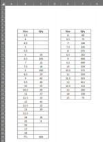
I am trying to apply the logic below to a code in VBA. Please see the attached screenshot of the excel screen for an added visual. In essence, if the specific size qty in column C is greater than it's corresponding size qty in column F, I need the value of column F to be reflected in column C (overriding the previous qty in column C with the value from column F). This is because the qty in column C cannot exceed the qty in column F.

If the VBA makes a change to column C, I need to change the font of the cell within column C to red, to visually indicate to a user that it has been changed. The logic would start at cell E8 (size 6, 60 qty) and work it's way down the list until it has reached cell E24 (size 15, 73 qty)

I thought using Index Match would be a good way to compare the size quantities, while also using an If formula to identify whether or not the qty in column C is > the qty in column F. However, Index Match doesn't get me the location of the cell, in which I would feed into the If formula. I am able to eye ball it in this example but that isn't a successful long term strategy, or one that I can automate this process with. (I converted these formulas over to VBA, but again, I don't think this is the correct path I should be taking - so probably disregard the below pieces of code)

= "=INDEX(C:C,MATCH(E8,B:B,0))"
= "=IF(C13>F8,F8,C13)"

Would love to hear your thoughts

 

[fadee2]

hi Oregon92,

Welcome to Board.

To use a formula I would suggest using index and match to return the matching values in column D. Because if you do try to change column C itself, then circular reference error will popup. Then use conditional formatting to highlight the cells that do not match.

=IFERROR(IF(J2<>INDEX($N$2:N11,MATCH(I2,$M$2:$M$11,0)),INDEX($N$2:N11,MATCH(I2,$M$2:$M$11,0))),"")

for vba, try the following code:

Dim rng As Range

Set rng = Sheets("sheet1").Range("v:v")

lr1 = Cells(Rows.Count, 18).End(xlUp).Row

    For x = 2 To lr1

        If Not IsError(Application.Match(Cells(x, 18), rng, 0)) Then
        s = Application.WorksheetFunction.Match(Cells(x, 18), rng, 0)

                If Cells(x, 19).Text <> Cells(s, 23).Text Then
                                   
                    Cells(x, 19) = Cells(s, 23)
                    Cells(x, 19).Font.Color = vbRed
                End If
        End If
    Next x

*change columns as per your needs

hth....

 

[Oregon92]

hi Oregon92,

Welcome to Board.

To use a formula I would suggest using index and match to return the matching values in column D. Because if you do try to change column C itself, then circular reference error will popup. Then use conditional formatting to highlight the cells that do not match.

=IFERROR(IF(J2<>INDEX($N$2:N11,MATCH(I2,$M$2:$M$11,0)),INDEX($N$2:N11,MATCH(I2,$M$2:$M$11,0))),"")

View attachment 41661

for vba, try the following code:

Dim rng As Range

Set rng = Sheets("sheet1").Range("v:v")

lr1 = Cells(Rows.Count, 18).End(xlUp).Row

    For x = 2 To lr1

        If Not IsError(Application.Match(Cells(x, 18), rng, 0)) Then
        s = Application.WorksheetFunction.Match(Cells(x, 18), rng, 0)

                If Cells(x, 19).Text <> Cells(s, 23).Text Then
                                  
                    Cells(x, 19) = Cells(s, 23)
                    Cells(x, 19).Font.Color = vbRed
                End If
        End If
    Next x

View attachment 41662


*change columns as per your needs

hth....

Thank you very much for your help! This worked excellent! I only had to adjust one line:

From: If Cells(x, 19).Text <> Cells(s, 23).Text Then
To: If Cells(x, 19).Value > Cells(s, 23).Value Then 'changed .Text to .Value and changed <> to >

Thank you again, so much! It's remarkable how you are able to view something like this, picture how it might work, and come up with something so quickly that does exactly what it's intended to do. You're a wizard!

 

[fadee2]

You are very welcome..... Glad to help....