Exclude from conditional formatting

commoguy_2010

New Member
Joined
Aug 13, 2016
Messages
7
Good day everyone,

I have an academic rating spreadsheet where students are ranked in the top 10%, 15% and 40%. So right now 3 conditional formatting rules. Each category of rating is recognized during their graduation and on their final graduation certification. However if the student has any thing negative they become ineligible for recognition.

So on my spreadsheet I have a column that indicates if they are ineligible for honors. I want to take the data from that column and use it to determine if they can be counted in my conditional formatting. So if there is an “x” in column B , exclude it from the conditional formatting.

Thanks for taking the time to read! Any help is greatly appreciated!
 

Excel Facts

Workdays for a market open Mon, Wed, Friday?
Yes! Use "0101011" for the weekend argument in NETWORKDAYS.INTL or WORKDAY.INTL. The 7 digits start on Monday. 1 means it is a weekend.
What are the actual conditions are you currently using as they display (if you use the boards XL2BB addin there is an option to display them in the thread or take a screenshot)?
 
Upvote 0
Since you just want the new rule to shutdown the other rules if col B = "x', you can create a new formula-based rule for 'col B = "x", and make it the first rule. Be sure to check the 'Stop If True' box'.

1701707935542.png
 
Upvote 0
What are the actual conditions are you currently using as they display (if you use the boards XL2BB addin there is an option to display them in the thread or take a screenshot)?
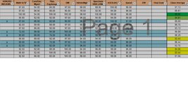
This is what I am working with. Also if a student is deemed to be ineligible, then it would skip to the next eligible with the next higher grade.
 

Attachments

  • Excel SS.jpg
    Excel SS.jpg
    161.4 KB · Views: 6
Upvote 0
Since you just want the new rule to shutdown the other rules if col B = "x', you can create a new formula-based rule for 'col B = "x", and make it the first rule. Be sure to check the 'Stop If True' box'.

View attachment 102914
Thank you! This worked. However, when I put an "X" in a column it simply takes it away. I need it to go to the next highest eligible grade.

So if Student A has a 99% and receives negative remarks, then student B with a 98% would then move to that top slot.
 
Upvote 0
I need it to go to the next highest eligible grade.

Not to be picky, but you said something else in your original post.
So if there is an “x” in column B , exclude it from the conditional formatting.

Just replace the formula in my example (=$B2="x") with whatever formula gives you the True/False result you need to activate whichever one of formats you need. Now if your next question is 'how do I do that' you will need to post specific and detailed information about your existing rules and their behavior if b = "x". Whether or not the new requirement can be merged with your existing rules depends on specifics. Because no one likes working with images like you posted above (the data and the CF rules cannot be imported for experimentation), the best way to do that is to follow @MARK858's suggestion above and use the free xl2BB add-in tool to post the same range you included in your image. That will let us see and work with the data and the conditional formatting rules for the range in question. If there is a question of proprietary data, then make up a sample worksheet with the same rules and use xl2BB to post that.
 
Upvote 0
Thank you! This worked. However, when I put an "X" in a column it simply takes it away. I need it to go to the next highest eligible grade.

So if Student A has a 99% and receives negative remarks, then student B with a 98% would then move to that top slot.

Not to be picky, but you said something else in your original post.


Just replace the formula in my example (=$B2="x") with whatever formula gives you the True/False result you need to activate whichever one of formats you need. Now if your next question is 'how do I do that' you will need to post specific and detailed information about your existing rules and their behavior if b = "x". Whether or not the new requirement can be merged with your existing rules depends on specifics. Because no one likes working with images like you posted above (the data and the CF rules cannot be imported for experimentation), the best way to do that is to follow @MARK858's suggestion above and use the free xl2BB add-in tool to post the same range you included in your image. That will let us see and work with the data and the conditional formatting rules for the range in question. If there is a question of proprietary data, then make up a sample worksheet with the same rules and use xl2BB to post that.
My apologies for the additional question, I had assumed Excel would automatically adjust and then appropriately highlight the next higher ranking, eligible student.

Unfortunately I am unable to add the useable screenshot due to this being done on a Government network. I have tried and it keeps failing. Ill keep working it and try to post again once I can use the addon you guys mentioned. Thank you.
 
Upvote 0

Forum statistics

Threads
1,215,079
Messages
6,123,009
Members
449,093
Latest member
ikke

We've detected that you are using an adblocker.

We have a great community of people providing Excel help here, but the hosting costs are enormous. You can help keep this site running by allowing ads on MrExcel.com.
Allow Ads at MrExcel

Which adblocker are you using?

Disable AdBlock

Follow these easy steps to disable AdBlock

1)Click on the icon in the browser’s toolbar.
2)Click on the icon in the browser’s toolbar.
2)Click on the "Pause on this site" option.
Go back

Disable AdBlock Plus

Follow these easy steps to disable AdBlock Plus

1)Click on the icon in the browser’s toolbar.
2)Click on the toggle to disable it for "mrexcel.com".
Go back

Disable uBlock Origin

Follow these easy steps to disable uBlock Origin

1)Click on the icon in the browser’s toolbar.
2)Click on the "Power" button.
3)Click on the "Refresh" button.
Go back

Disable uBlock

Follow these easy steps to disable uBlock

1)Click on the icon in the browser’s toolbar.
2)Click on the "Power" button.
3)Click on the "Refresh" button.
Go back
Back
Top