Filter across multiple columns, but without using helper column

[ellison]

Hi, I'm trying to filter for a single criteria across multiple columns.

- I'd normally use a helper column to concatenate the relevant fields together.
- Then copy / paste special / paste the "values" into the same helper column in order that they can be filtered.
- For example

Row	Model	Material	Colour	Helper
2	XYZ789	Wood	Silver	XYZ789;Wood;Silver
3	ABC123-4	Plastic	Black	ABC123-4;Plastic;Black
4	14CV56576		Wood	14CV56576;Wood

EG If we wanted to view any row of info which contained "Wood", then the filter would show Rows 2 and 4.

Is there a way of doing this where I can make this work without having to copy / paste special / paste "values in the helper column? (otherwise my fat fingers seem to be causing all sorts of errors!).

Huge thanks

 

[Michael M]

Why not simply fix the data set so that the items are in the correct columns.....unles of course, wood IS a colour

 

[Michael M]

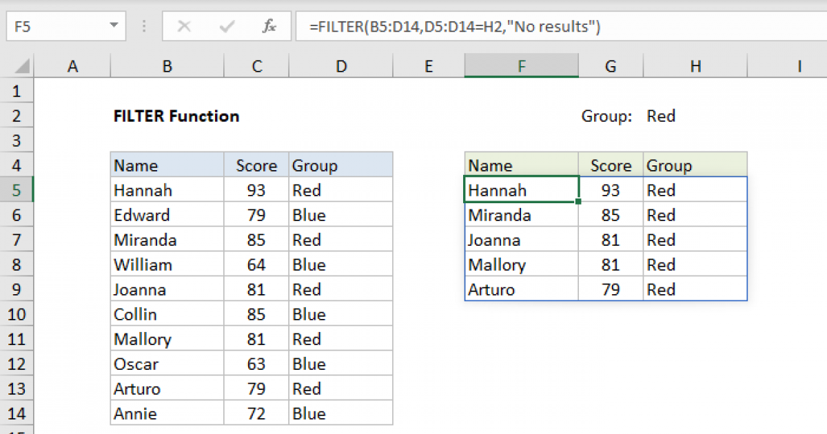
I also see your using 365, which contains a new function called =FILTER
Have a look here for examples, especially about halfway down where it says "more Than one Criteria"

FILTER Function

The Excel FILTER function is used to extract matching values from data based on one or more conditions. The output from FILTER is dynamic. If source data or criteria change, FILTER will return a new set of results. This makes FILTER a flexible way to isolate and inspect data without altering the...

exceljet.net

 

[ellison]

Why not simply fix the data set so that the items are in the correct columns.....unles of course, wood IS a colour

Would love to, but these are external reports that we have to tidy up. Every month. Joy!

 

[ellison]

I also see your using 365, which contains a new function called =FILTER
Have a look here for examples, especially about halfway down where it says "more Than one Criteria"

FILTER Function

The Excel FILTER function is used to extract matching values from data based on one or more conditions. The output from FILTER is dynamic. If source data or criteria change, FILTER will return a new set of results. This makes FILTER a flexible way to isolate and inspect data without altering the...

exceljet.net

a-ha, I'd been looking at that one...

The new FILTER option seems to copy the filtered data into a different location.

Whereas I need to be editing the data in its original location. (And some rows of data need multiple corrections).

Hope this helps

 

[Michael M]

This assumes that the data is in columns A-D.

Sub MM1()
Dim r As Long
For r = 4 To 2 Step -1
    If Cells(r, 2).Value = "Wood" Or Cells(r, 3) = "Wood" Then
        Rows(r).EntireRow.Hidden = False
        Else
        Rows(r).EntireRow.Hidden = True
    End If
Next r
End Sub

 

[ellison]

Hi Michael, huge thanks for the code!
I seem to be having a couple of gremlins, sorry.
I've entered this as a UDF.
Then when I ran it, Excel jumped to cell MM1 (as opposed to running the macro)

I hit Alt + F8 a second time and the data filtered (but missed out a row that would include "wood").

Which would leave my other gremlin: I couldn't see how to remove the filter to get back to the raw data?

(And last, could the code run the filter from the contents of a cell address eg "H1"? That way I could change the contents of cell H1 to "wood" or "plastic" etc without having to change the actual code)

Many thanks for your help Michael


When I run the mac

 

[Michael M]

You would have to rename it if you used it as a function, but you could simply run it usinf F8 and selecting the macro MM1
To get back to raw data simply click in the Intersect of rows and columns )just above row 1 and then right click and select "Unhide"
To use "H1" try...

Sub MM1()
Dim r As Long, rng as range
set rng = cells(1,8)
For r = 4 To 2 Step -1
    If Cells(r, 2).Value = rng Or Cells(r, 3) = rng Then
        Rows(r).EntireRow.Hidden = False
        Else
        Rows(r).EntireRow.Hidden = True
    End If
Next r
End Sub

 

[ellison]

Thanks Michael...
On the plus side, I renamed the UDF to Dynamic Test (rather than MM) and it worked with cell input "H1"- although still some gremlins.

- On the down side, it seems to be case dependent? (could this be avoided?)
- And sorry to say that it didn't pick up the second row of info (although it did pick up the first!)
- Also, I'm going to have to be toggling the filter on and off (a lot, deep joy !)....
- Is there a way of making that a little quicker / easier rather than clicking on the intersect?

Thanks again

 

[ellison]

Hi,

I tried going back to seeing if using functions in a helper column would work.
But tried different methods of joining them together .... No luck I'm afraid

dynamic-test.xlsx
	A	B	C	D	E	F
1	Row	Make	Model	Colour	Helper	Helper-to-view-function
2	2	one	two	three	2onetwothree	#=B2&C2&D2&E2
3	3	one	two	Black	3onetwoBlack	#=B3&C3&D3&E3
4	4	14CV56576		Wood	414CV56576Wood	#=B4&C4&D4&E4
5	5	one	two	three	5onetwothree	#=CONCATENATE(B5,C5,D5,E5)
6	6	one	two	Black	6onetwoBlack	#=CONCATENATE(B6,C6,D6,E6)
7	7	14CV56576		Wood	714CV56576Wood	#=CONCATENATE(B7,C7,D7,E7)
8	8	one	two	three	one;two;three	#=TEXTJOIN(";",TRUE,C8:E8)
9	9	one	two	Black	one;two;Black	#=TEXTJOIN(";",TRUE,C9:E9)
10	10	14CV56576		Wood	14CV56576;Wood	#=TEXTJOIN(";",TRUE,C10:E10)
Sheet3

Cell Formulas
Range	Formula
E2:E4	E2	=A2&B2&C2&D2
E5:E7	E5	=CONCATENATE(A5,B5,C5,D5)
E8:E10	E8	=TEXTJOIN(";",TRUE,B8:D8)

If anybody has any suggestions, I'm all ears!

PS the sheet had a filter set on it