Filter Function Alternate for Excel 2016

[mwaseeuddin]

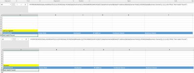
I have created search engine in Office 365 Excel Using Filter Function, however, it's not working in Excel 2016

Please find below Formula and please help me with a formula which works in Excel 2016.

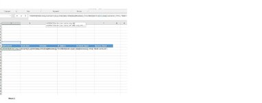
=_xlfn._xlws.FILTER(Data,ISNUMBER(SEARCH($A$7,Data[Server Role]&Data[Hostname]&Data[IP Address]))=TRUE,"Not match found")

Many thanks in advance.

 

[KRice]

In Excel 2016, you won't have the same convenience of automatically spilling the results like FILTER does. Instead, a formula determines the indexed rows that satisfy the matching criteria (AGGREGATE), and INDEX is used to extract those rows and columns (shown in the last array). The formula needs to be pulled down until blanks appear, which indicates that all matching items have been found.

MrExcel_20240112.xlsx
	A	B	C	D	E	F	G	H	I	J
7	aapple192.0.2.1	a	apple	y	192.0.2.1		Server Role	Hostname	Other Info	IP Address
8		a	apple	p	192.0.2.1		a	apple	x	192.0.2.2
9		a	apple	s	192.0.2.1		a	apple	y	192.0.2.1
10							a	mango	z	192.0.2.1
11							a	apple	p	192.0.2.1
12	aapple192.0.2.1	a	apple	y	192.0.2.1		b	mango	q	192.0.2.2
13		a	apple	p	192.0.2.1		b	mango	r	192.0.2.2
14		a	apple	s	192.0.2.1		a	apple	s	192.0.2.1
15
16
Sheet4

Cell Formulas
Range	Formula
B7:E9	B7	=FILTER(Data,ISNUMBER(SEARCH($A$7,Data[Server Role]&Data[Hostname]&Data[IP Address]))=TRUE,"Not match found")
B12:E16	B12	=IFERROR(INDEX(Data,AGGREGATE(15,6,(ROW(Data)-ROW(Data[#Headers]))/ISNUMBER(SEARCH($A$12,Data[Server Role]&Data[Hostname]&Data[IP Address])),ROWS(B$12:B12)),{1,2,3,4}),"")
Dynamic array formulas.

 

[mwaseeuddin]

Dear Kirk,

Many Thanks for your reply.

I followed your instructions, however, still it's not working, please see below formula and attached screen shots.
=IFERROR(INDEX(Data,AGGREGATE(15,6,(ROW(Data)-ROW(Data[#Headers]))/ISNUMBER(SEARCH($A$7,Data[Hostname]&Data[IP Address]&Data[Server Role])),ROWS(Data[Business Owner])),{1,2,3,4})=TRUE,"Not match found")

 

[Peter_SSs]

@KRice
Isn't your suggestion still employing a spill feature (across each result row) that would not be available in 2016?

@mwaseeuddin
Welcome to the MrExcel board!
We don't know anything about your layout, particularly the table 'Data'. Can you provide small a sample (with any sensitive information disguised) including the expected results with XL2BB? That way we would have some idea of, not only the data, but the layout/structure of the table & result requirements.

 

[mwaseeuddin]

Dear Peter,

In Sheet 1 I created a table and named Data and in Sheet2 I have same headers a Data Table and I want search in row A7 and formula should fetch information from Data table in Sheet1.

Please see the attached screen shot for more information.

Many thanks for your help.
Mohammed.

 

[mwaseeuddin]

Please see the attached Screen Shots.

 

[KRice]

Ahh...right you are, @Peter_SSs...thank you. I had a hard-wired array to pull the columns, which is a spill feature.

@mwaseeuddin, here is a similar version, but the formula needs to be dragged throughout the results table. Also, please see Peter's request. Knowing what your source table looks like would help greatly. Also, is there some reason why you are beginning your search with a single concatenated term (Server Role & Hostname & IP Address)? Do you initially know each of those as individual terms? If so, other formula approaches could be taken.

MrExcel_20240117.xlsx
	A	B	C	D	E	F	G	H	I	J
1
2	aapple192.0.2.1	a	apple	y	192.0.2.1		Server Role	Hostname	Other Info	IP Address
3		a	apple	p	192.0.2.1		a	apple	x	192.0.2.2
4		a	apple	s	192.0.2.1		a	apple	y	192.0.2.1
5							a	mango	z	192.0.2.1
6							a	apple	p	192.0.2.1
7							b	mango	q	192.0.2.2
8							b	mango	r	192.0.2.2
9							a	apple	s	192.0.2.1
Sheet4

Cell Formulas
Range	Formula
B2:E6	B2	=IFERROR(INDEX(Data,AGGREGATE(15,6,(ROW(Data)-ROW(Data[#Headers]))/ISNUMBER(SEARCH($A$2,Data[[Server Role]:[Server Role]]&Data[[Hostname]:[Hostname]]&Data[[IP Address]:[IP Address]])),ROWS($2:2)),COLUMNS($B:B)),"")

 

[Peter_SSs]

Please see the attached Screen Shots.

Unfortunately we cannot copy from screen shots to test. Please see my previous post about XL2BB as we can easily copy from that.

Firstly here is my sample data (slightly changed from yours) ..

mwaseeuddin.xlsm
	A	B	C	D	E	F	G
1	Environment	Server_Role	Hostname	IP_Address	Technical_Owner	Business Owner
2	First	Second	Sixth	Seventh	Eight	BO 1
3	Third	Fourth	Fifth	First	Eleventh	BO 2
4	Third	Fourth	Fifth	First	Eleventh	BO 3
5	Third	Fourth	Fifth	First	Eleventh	BO 4
6	Third	Fourth	Fifth	First	Eleventh	BO 5
7	Third	Fourth	Fifth	First	Eleventh	BO 6
8	Third	Fourth	Fifth	First	Eleventh	BO 7
9	Third	Fourth	Fifth	First	Eleventh	BO 8
10	First	Second	Sixth	Seventh	Eight	BO 9
11	Third	Fourth	Fifth	First	Eleventh	BO 10
12	Third	Fourth	Fifth	First	Eleventh	BO 11
13	Third	Fourth	Fifth	First	Eleventh	BO 12
14	Third	Fourth	Fifth	First	Eleventh	BO 13
15	Third	Fourth	Fifth	First	Eleventh	BO 14
16	Third	Fourth	Fifth	First	Eleventh	BO 15
17	Third	Fourth	Fifth	First	Eleventh	BO 16
18	Third	Fourth	Fifth	First	Eleventh	BO 17
19	Third	Fourth	Fifth	First	Eleventh	BO 18
20	Third	Fourth	Fifth	First	Eleventh	BO 19
21	Third	Fourth	Fifth	First	Eleventh	BO 20
22	Third	Fourth	Fifth	First	Eleventh	BO 21
23	Third	Fourth	Fifth	First	Eleventh	BO 22
24	Third	Fourth	Fifth	First	Eleventh	BO 23
25	Third	Fourth	Fifth	First	Eleventh	BO 24
Sheet1

.. and 365 results with a formula similar to the one you showed in post 1

mwaseeuddin.xlsm
	A	B	C	D	E	F
7	SecondSixthSeventh
8	Environment	Server_Role	Hostname	IP_Address	Technical_Owner	Business Owner
9	First	Second	Sixth	Seventh	Eight	BO 1
10	First	Second	Sixth	Seventh	Eight	BO 9
11
Sheet2

Cell Formulas
Range	Formula
A9:H10	A9	=FILTER(Data,ISNUMBER(SEARCH($A$7,Data[Server_Role]&Data[Hostname]&Data[IP_Address]))=TRUE,"Not match found")
Dynamic array formulas.

This is how I would approach the problem with Excel 2016.
Add two new columns to the table as shown below. Once the columns have been added and formulas inserted, these columns could be hidden if you want the table to look exactly like it did before.

mwaseeuddin.xlsm
	A	B	C	D	E	F	G	H	I
1	Environment	Server_Role	Hostname	IP_Address	Technical_Owner	Business Owner	SR_HN_IP	Idx
2	First	Second	Sixth	Seventh	Eight	BO 1	SecondSixthSeventh	1
3	Third	Fourth	Fifth	First	Eleventh	BO 2	FourthFifthFirst	1
4	Third	Fourth	Fifth	First	Eleventh	BO 3	FourthFifthFirst	1
5	Third	Fourth	Fifth	First	Eleventh	BO 4	FourthFifthFirst	1
6	Third	Fourth	Fifth	First	Eleventh	BO 5	FourthFifthFirst	1
7	Third	Fourth	Fifth	First	Eleventh	BO 6	FourthFifthFirst	1
8	Third	Fourth	Fifth	First	Eleventh	BO 7	FourthFifthFirst	1
9	Third	Fourth	Fifth	First	Eleventh	BO 8	FourthFifthFirst	1
10	First	Second	Sixth	Seventh	Eight	BO 9	SecondSixthSeventh	2
11	Third	Fourth	Fifth	First	Eleventh	BO 10	FourthFifthFirst	2
12	Third	Fourth	Fifth	First	Eleventh	BO 11	FourthFifthFirst	2
13	Third	Fourth	Fifth	First	Eleventh	BO 12	FourthFifthFirst	2
14	Third	Fourth	Fifth	First	Eleventh	BO 13	FourthFifthFirst	2
15	Third	Fourth	Fifth	First	Eleventh	BO 14	FourthFifthFirst	2
16	Third	Fourth	Fifth	First	Eleventh	BO 15	FourthFifthFirst	2
17	Third	Fourth	Fifth	First	Eleventh	BO 16	FourthFifthFirst	2
18	Third	Fourth	Fifth	First	Eleventh	BO 17	FourthFifthFirst	2
19	Third	Fourth	Fifth	First	Eleventh	BO 18	FourthFifthFirst	2
20	Third	Fourth	Fifth	First	Eleventh	BO 19	FourthFifthFirst	2
21	Third	Fourth	Fifth	First	Eleventh	BO 20	FourthFifthFirst	2
22	Third	Fourth	Fifth	First	Eleventh	BO 21	FourthFifthFirst	2
23	Third	Fourth	Fifth	First	Eleventh	BO 22	FourthFifthFirst	2
24	Third	Fourth	Fifth	First	Eleventh	BO 23	FourthFifthFirst	2
25	Third	Fourth	Fifth	First	Eleventh	BO 24	FourthFifthFirst	2
Sheet1

Cell Formulas
Range	Formula
G2:G25	G2	=[@[Server_Role]]&[@Hostname]&[@[IP_Address]]
H2:H25	H2	=COUNTIF(INDEX([SR_HN_IP],1):[@[SR_HN_IP]],Sheet2!A$7)

Now in cell A9 of Sheet2 use this formula and copy it across and down

=IFNA(INDEX(Data[Environment],MATCH(ROWS(A$9:A9),Data[[Idx]:[Idx]],0)),"")

Here are my results

mwaseeuddin.xlsm
	A	B	C	D	E	F
7	SecondSixthSeventh
8	Environment	Server_Role	Hostname	IP_Address	Technical_Owner	Business Owner
9	First	Second	Sixth	Seventh	Eight	BO 1
10	First	Second	Sixth	Seventh	Eight	BO 9
11
12
Sheet2