Filtering from one workbook, pasting into another

jalrs

Active Member
Joined
Apr 6, 2022
Messages
300
Office Version
  1. 365
Platform
  1. Windows
Hello guys,

I'm new to VBA and therefore i need some help. I would be glad if i found it here.
So, my problem is: I runned a code after doing my search here, but the code misses on something, after i did my changes and debug it. Im filtering from a sheet called "Stock Trânsito" in Workbook1 to paste on a sheet called "pendentes" on a workbook called "STTApoioSP". When i run the code, instead of pasting into cell "A2" it pastes into cell "A21" and brings a value that doesnt match the criteria filter.

My code:

Sub filterAPOIOSP()

ThisWorkbook.Worksheets("Stock Trânsito").Activate

Dim lastrow As Long, lastrow2 As Long

lastrow = Cells(Rows.Count, "A").End(xlUp).Row
lastrow2 = Workbooks("STTApoioSP.xlsm").Sheets("pendentes").Cells(Rows.Count, "A").End(xlUp).Row

With ActiveSheet.Range("A6:AV" & lastrow)
.AutoFilter Field:=46, Criteria1:="Apoio SP", Operator:=xlFilterValues
.SpecialCells(xlCellTypeVisible).Copy Workbooks("STTApoioSP.xlsm").Worksheets("pendentes").Range("A2" & lastrow2)

End With

ActiveSheet.AutoFilterMode = False

End Sub


Additional questions:
1- If i want to add criteria2, how should i add it into the code?
2- how can i add a specific column from my workbook to this new one? i mean, where do i write it on the code?

thanks in advance!
 
Hello Kevin, hope all is good with you.

Coming back here, since you helped me with this. What would i add to the code if i want to copy sets of columns? instead of one set + one column like we did.

I tried with "with" like you showed on your suggestion but gave me an error, therefore i removed it, and got back to our starting point

Context of situation, current code:
VBA Code:
Sub filtroLoja()

    Dim wb1 As Workbook, wb2 As Workbook
    Dim ws1 As Worksheet, ws2 As Worksheet
   
    Set wb1 = ThisWorkbook
    Set wb2 = Workbooks("Template.xlsm")
   
    Set ws1 = wb1.Worksheets("Stock Trânsito")
    Set ws2 = wb2.Worksheets("Loja")
   
    ws2.UsedRange.Offset(1).ClearContents
   
    Dim lr1 As Long, lr2 As Long
   
    lr1 = ws1.Cells(Rows.Count, 1).End(3).Row
    lr2 = ws2.Cells(Rows.Count, 1).End(3).Row + 1
   
    With ws1.Range("A5:AV" & lr1)
   
        .AutoFilter 46, "Loja"
        .AutoFilter 47 "Em tratamento"
        .Offset(1).Copy ws2.Cells(lr2, 1)
       
        With ws1.Range("BH6:BH" & lr1)
       
           .Copy ws2.Cells(2, 49)
          
        End With
       
        .AutoFilter
       
    End With
   
    lr2 = ws2.Cells.Find("*", , xlFormulas, , 1, 2).Row + 1
    ws2.Range("A" & lr2 & ":A1001").EntireRow.Delete
   
End Sub

What i want: i don't want to copy all the way from A5:AV, but instead i want: A5:T + W5:AC + AF5:AV + BH

Thanks!
 
Upvote 0

Excel Facts

How to show all formulas in Excel?
Press Ctrl+` to show all formulas. Press it again to toggle back to numbers. The grave accent is often under the tilde on US keyboards.
OK, try this. Let me know how it goes, and I'll get back to you (tomorrow).

VBA Code:
Option Explicit
Sub jalrs6()
    Dim wb1 As Workbook, wb2 As Workbook
    Dim ws1 As Worksheet, ws2 As Worksheet
    Set wb1 = ThisWorkbook
    Set wb2 = Workbooks("STTApoioSP.xlsm")
    
    Set ws1 = wb1.Worksheets("Stock Trânsito")
    Set ws2 = wb2.Worksheets("pendentes")
    
    ws2.UsedRange.Offset(1).ClearContents
    
    Dim lr1 As Long, lr2 As Long
    lr1 = ws1.Cells(Rows.Count, 1).End(3).Row
    lr2 = ws2.Cells(Rows.Count, 1).End(3).Row + 1
    
    With ws1.Range("A5:AV" & lr1)
        .AutoFilter 46, "Loja"
        .AutoFilter 47, "Em tratamento"
            With ws1
                .Range("A5:T" & lr1).Offset(1).Copy ws2.Cells(2, 1)
                .Range("W5:AC" & lr1).Offset(1).Copy ws2.Cells(2, 21)
                .Range("AF5:AV" & lr1).Offset(1).Copy ws2.Cells(2, 28)
                .Range("BH5:BH" & lr1).Offset(1).Copy ws2.Cells(2, 45)
            End With
        .AutoFilter
    End With
    
    lr2 = ws2.Cells.Find("*", , xlFormulas, , 1, 2).Row + 1
    ws2.Range("A" & lr2 & ":A1001").EntireRow.Delete
End Sub
 
Upvote 0
OK, try this. Let me know how it goes, and I'll get back to you (tomorrow).

VBA Code:
Option Explicit
Sub jalrs6()
    Dim wb1 As Workbook, wb2 As Workbook
    Dim ws1 As Worksheet, ws2 As Worksheet
    Set wb1 = ThisWorkbook
    Set wb2 = Workbooks("STTApoioSP.xlsm")
   
    Set ws1 = wb1.Worksheets("Stock Trânsito")
    Set ws2 = wb2.Worksheets("pendentes")
   
    ws2.UsedRange.Offset(1).ClearContents
   
    Dim lr1 As Long, lr2 As Long
    lr1 = ws1.Cells(Rows.Count, 1).End(3).Row
    lr2 = ws2.Cells(Rows.Count, 1).End(3).Row + 1
   
    With ws1.Range("A5:AV" & lr1)
        .AutoFilter 46, "Loja"
        .AutoFilter 47, "Em tratamento"
            With ws1
                .Range("A5:T" & lr1).Offset(1).Copy ws2.Cells(2, 1)
                .Range("W5:AC" & lr1).Offset(1).Copy ws2.Cells(2, 21)
                .Range("AF5:AV" & lr1).Offset(1).Copy ws2.Cells(2, 28)
                .Range("BH5:BH" & lr1).Offset(1).Copy ws2.Cells(2, 45)
            End With
        .AutoFilter
    End With
   
    lr2 = ws2.Cells.Find("*", , xlFormulas, , 1, 2).Row + 1
    ws2.Range("A" & lr2 & ":A1001").EntireRow.Delete
End Sub
Works great!

Thanks Kevin!
 
Upvote 0
Hello @kevin9999 , I hope everything is good with you.

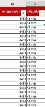
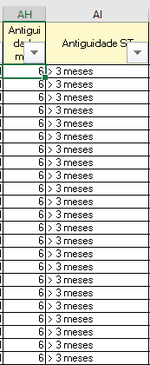
I was preparing for my presentation of the project and noticed that on some columns it is copying the source worksheet formula. This said, the destination column will have the wrong values, since we are copying a specific range from source sheet and not all columns. Please see attachments. I also highlighted where I think the problem resides as a comment

VBA Code:
Option Explicit
Sub filtromacro1()

Application.ScreenUpdating = False
Application.DisplayAlerts = False

Dim wb1 As Workbook, wb2 As Workbook
Dim ws1 As Worksheet, ws2 As Worksheet, ws3 As Worksheet
Dim lr1 As Long, lr2 As Long, lr3 As Long, lr4 As Long, i As Long
Dim mypath As String, docname As String, valorfiltro As String

Set wb1 = ThisWorkbook
Set ws1 = wb1.Worksheets("Stock")
Set ws2 = wb1.Worksheets("MACRO 1")

lr1 = ws1.Cells(Rows.Count, "A").End(xlUp).Row
lr2 = ws2.Cells(Rows.Count, "A").End(xlUp).Row

ws2.Activate

    For i = 2 To lr2
       
        valorfiltro = Cells(i, 1).Value
       
        Workbooks.Open Filename:=ThisWorkbook.Path & "\Temp\ST_TEMPLATE_" & Cells(i, 1).Value & ".xlsx"
       
        Set wb2 = Workbooks("ST_TEMPLATE_" & valorfiltro & ".xlsx")
       
        Set ws3 = wb2.Worksheets("Pendentes")
       
        ws3.Activate
       
        ws3.UsedRange.Offset(1).ClearContents
       
        lr3 = ws3.Cells(Rows.Count, "A").End(xlUp).Row + 1
       
        ws1.Activate
       
        With ws1.Range("A5:AV" & lr1)
       
            .AutoFilter 46, valorfiltro
            .AutoFilter 47, "Em tratamento"
           
            With ws1
       
            .Range("A6:AV" & lr1).Copy ws3.Cells(2, 1) ' i think the problem is here most likely, just don't know how to sort it out
            .Range("BH6:BH" & lr1).Copy ws3.Cells(2, 49) ' same as above line
           
            End With
           
            .AutoFilter
       
        End With
       
        lr3 = ws3.Cells.Find("*", , xlFormulas, , 1, 2).Row + 1
        ws3.Range("A" & lr3 & ":A1001").EntireRow.Delete
       
        wb2.Activate
       
        ws3.Activate
       
        lr4 = Cells(Rows.Count, "AT").End(xlUp).Row
       
        If lr4 > 1 Then
       
            Range("AY2:AY" & lr4).FormulaR1C1 = _
            "=IF(RC[-1]="""","""",VLOOKUP(RC[-1],TAB_FDB!C[-50]:C[-49],2,0))"
           
        End If
       
        ws3.Protect Password:="blabla", _
        DrawingObjects:=True, _
        Contents:=True, _
        Scenarios:=True, _
        UserInterfaceOnly:=True, _
        AllowFormattingCells:=False, _
        AllowFormattingColumns:=False, _
        AllowFormattingRows:=False, _
        AllowInsertingColumns:=False, _
        AllowInsertingRows:=False, _
        AllowInsertingHyperlinks:=False, _
        AllowDeletingColumns:=False, _
        AllowDeletingRows:=False, _
        AllowSorting:=True, _
        AllowFiltering:=False, _
        AllowUsingPivotTables:=False

        mypath = ThisWorkbook.Path & "\Anexos\"
           
        wb1.Activate
       
        ws2.Activate
       
        docname = Cells(i, 5).Value
       
        wb2.Activate
       
        ws3.Activate
       
        ActiveWorkbook.SaveAs Filename:=mypath & docname & ".xlsx", FileFormat:=xlOpenXMLWorkbook
   
        ActiveWorkbook.Close
       
    Next i
   
Application.DisplayAlerts = True
Application.ScreenUpdating = True

End Sub

EDIT: Already tried adding
Rich (BB code):
.PasteSpecial Paste:=xlPasteValues
but returns an error message

Thanks Kevin
 

Attachments

  • destvalues.png
    destvalues.png
    8.6 KB · Views: 1
  • sourcevalues.png
    sourcevalues.png
    7.2 KB · Views: 1
Last edited:
Upvote 0
Hello @kevin9999 , I hope everything is good with you.

I was preparing for my presentation of the project and noticed that on some columns it is copying the source worksheet formula. This said, the destination column will have the wrong values, since we are copying a specific range from source sheet and not all columns. Please see attachments. I also highlighted where I think the problem resides as a comment

VBA Code:
Option Explicit
Sub filtromacro1()

Application.ScreenUpdating = False
Application.DisplayAlerts = False

Dim wb1 As Workbook, wb2 As Workbook
Dim ws1 As Worksheet, ws2 As Worksheet, ws3 As Worksheet
Dim lr1 As Long, lr2 As Long, lr3 As Long, lr4 As Long, i As Long
Dim mypath As String, docname As String, valorfiltro As String

Set wb1 = ThisWorkbook
Set ws1 = wb1.Worksheets("Stock")
Set ws2 = wb1.Worksheets("MACRO 1")

lr1 = ws1.Cells(Rows.Count, "A").End(xlUp).Row
lr2 = ws2.Cells(Rows.Count, "A").End(xlUp).Row

ws2.Activate

    For i = 2 To lr2
      
        valorfiltro = Cells(i, 1).Value
      
        Workbooks.Open Filename:=ThisWorkbook.Path & "\Temp\ST_TEMPLATE_" & Cells(i, 1).Value & ".xlsx"
      
        Set wb2 = Workbooks("ST_TEMPLATE_" & valorfiltro & ".xlsx")
      
        Set ws3 = wb2.Worksheets("Pendentes")
      
        ws3.Activate
      
        ws3.UsedRange.Offset(1).ClearContents
      
        lr3 = ws3.Cells(Rows.Count, "A").End(xlUp).Row + 1
      
        ws1.Activate
      
        With ws1.Range("A5:AV" & lr1)
      
            .AutoFilter 46, valorfiltro
            .AutoFilter 47, "Em tratamento"
          
            With ws1
      
            .Range("A6:AV" & lr1).Copy ws3.Cells(2, 1) ' i think the problem is here most likely, just don't know how to sort it out
            .Range("BH6:BH" & lr1).Copy ws3.Cells(2, 49) ' same as above line
          
            End With
          
            .AutoFilter
      
        End With
      
        lr3 = ws3.Cells.Find("*", , xlFormulas, , 1, 2).Row + 1
        ws3.Range("A" & lr3 & ":A1001").EntireRow.Delete
      
        wb2.Activate
      
        ws3.Activate
      
        lr4 = Cells(Rows.Count, "AT").End(xlUp).Row
      
        If lr4 > 1 Then
      
            Range("AY2:AY" & lr4).FormulaR1C1 = _
            "=IF(RC[-1]="""","""",VLOOKUP(RC[-1],TAB_FDB!C[-50]:C[-49],2,0))"
          
        End If
      
        ws3.Protect Password:="blabla", _
        DrawingObjects:=True, _
        Contents:=True, _
        Scenarios:=True, _
        UserInterfaceOnly:=True, _
        AllowFormattingCells:=False, _
        AllowFormattingColumns:=False, _
        AllowFormattingRows:=False, _
        AllowInsertingColumns:=False, _
        AllowInsertingRows:=False, _
        AllowInsertingHyperlinks:=False, _
        AllowDeletingColumns:=False, _
        AllowDeletingRows:=False, _
        AllowSorting:=True, _
        AllowFiltering:=False, _
        AllowUsingPivotTables:=False

        mypath = ThisWorkbook.Path & "\Anexos\"
          
        wb1.Activate
      
        ws2.Activate
      
        docname = Cells(i, 5).Value
      
        wb2.Activate
      
        ws3.Activate
      
        ActiveWorkbook.SaveAs Filename:=mypath & docname & ".xlsx", FileFormat:=xlOpenXMLWorkbook
  
        ActiveWorkbook.Close
      
    Next i
  
Application.DisplayAlerts = True
Application.ScreenUpdating = True

End Sub

EDIT: Already tried adding
Rich (BB code):
.PasteSpecial Paste:=xlPasteValues
but returns an error message

Thanks Kevin
The code I provided to you in post #42 did what you wanted it to: "Works great!" is what you said.

You have then made some significant changes to that code - and now it doesn't work for you.

Given that this is post #46, I suggest you start a new thread to resolve your problem.
 
Upvote 0

Forum statistics

Threads
1,214,982
Messages
6,122,581
Members
449,089
Latest member
Motoracer88

We've detected that you are using an adblocker.

We have a great community of people providing Excel help here, but the hosting costs are enormous. You can help keep this site running by allowing ads on MrExcel.com.
Allow Ads at MrExcel

Which adblocker are you using?

Disable AdBlock

Follow these easy steps to disable AdBlock

1)Click on the icon in the browser’s toolbar.
2)Click on the icon in the browser’s toolbar.
2)Click on the "Pause on this site" option.
Go back

Disable AdBlock Plus

Follow these easy steps to disable AdBlock Plus

1)Click on the icon in the browser’s toolbar.
2)Click on the toggle to disable it for "mrexcel.com".
Go back

Disable uBlock Origin

Follow these easy steps to disable uBlock Origin

1)Click on the icon in the browser’s toolbar.
2)Click on the "Power" button.
3)Click on the "Refresh" button.
Go back

Disable uBlock

Follow these easy steps to disable uBlock

1)Click on the icon in the browser’s toolbar.
2)Click on the "Power" button.
3)Click on the "Refresh" button.
Go back
Back
Top