Find 3 matches within 5 columns highlight and get summary

[motilulla]

Hello,

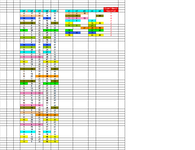
I got data base in the 5 columns in the D:H cells D6:H59 (my actually data base is in the range D6:H4108) I want to get highlighted 3 match within 5 columns in the any position and (optional is possible to get match count summary in the cells J6: N to down in the columns.

														Count 3 Match
			n1	n2	n3	n4	n5		n1	n2	n3	n4	n5	Total Find
			4	12	24	27	36		1	4	10			2
			1	4	10	19	23		1	10			48	4
			14	15	28	35	40		1	6	13			4
			12	20	21	45	48		4	9		21		2
			1	10	12	16	48		4			46	48	2
			3	8	12	29	43		5	9		21		2
			12	37	39	40	50				27	38	48	2
			10	28	40	47	48		10			47	48	2
			3	7	25	45	50		14	15		35		2
			6	9	15	25	38		18			46	48	2
			5	9	19	21	38
			5	7	14	20	49
			2	8	17	32	50
			14	15	25	35	47
			5	9	20	21	26
			10	20	22	24	31
			4	9	15	21	47
			5	27	31	40	42
			1	6	13	30	49
			13	24	26	47	49
			18	23	37	46	48
			11	14	24	25	29
			3	7	12	26	34
			1	10	17	33	48
			5	6	11	30	44
			8	15	26	30	48
			10	22	27	38	48
			7	17	20	35	50
			1	10	44	45	48
			10	25	41	47	48
			6	8	27	37	41
			12	13	17	22	43
			5	19	31	43	50
			1	6	13	22	28
			20	21	27	33	40
			3	9	20	30	42
			10	15	17	40	45
			10	13	20	33	41
			1	6	13	17	26
			1	10	29	38	48
			5	8	14	22	32
			1	4	10	41	45
			7	12	27	38	48
			15	25	26	40	41
			18	28	39	46	48
			9	23	29	41	49
			1	6	13	15	16
			5	25	32	37	43
			3	18	22	27	32
			4	9	14	21	27
			4	8	11	19	46
			4	12	25	46	48
			2	19	24	26	49
			4	5	39	46	48

For example the sample image is attached.

Thank you all.

I am using Excel 2000

Regards,
Moti

 

[KRice]

Here is one idea to consider. What makes this more difficult is that for every set of five numbers, there are 10 possible combinations that need to be considered. By using helper columns, you could explicitly list these combinations (see the table with blue heading) and then search the entire table of combinations for duplicates. The example here uses this approach, and to clarify which group of three will be taken from the five numbers, you will see an array of the form {1,1,1,0,0}, which means use the 1st, 2nd, and 3rd numbers and omit the 4th and 5th. These arrays change for each of the 10 columns and are (unfortunately) embedded in the formulas in three places. Since you are using Excel 2000, the use of the TEXTJOIN function, which I used here, is probably not an option, but you can accomplish exactly the same text strings using a construction like this:

=CONCATENATE(INDEX($D7:$H7,AGGREGATE(15,6,(COLUMN($D$6:$H$6)-COLUMN($C$6))/{1,1,1,0,0},1)),
        ,",",INDEX($D7:$H7,AGGREGATE(15,6,(COLUMN($D$6:$H$6)-COLUMN($C$6))/{1,1,1,0,0},2)),
        ,",",INDEX($D7:$H7,AGGREGATE(15,6,(COLUMN($D$6:$H$6)-COLUMN($C$6))/{1,1,1,0,0},3))
)

...which should work fine in Excel 2000.

This approach assumes that the original sets of five numbers are in sorted order, from least to greatest. For the sake of brevity, I've only shown five rows of numbers, and I've changed some of the original values so that some duplicates would be found. The duplicate counts are shown in the "Matches" table (green heading).

A VBA solution is probably preferred here, as the number of combinations and the fact that potential matches are spread across 10 columns complicates being able to extract a unique list of duplicates across those 10 columns. Perhaps someone has a clever way to do that. For now, I've used Conditional Formatting to search the table and highlight duplicates. In the example shown, some of the matches indicated by highlighting and counts>1 may not be obvious because the entire table is not shown.

MrExcel20210308.xlsx
	C	D	E	F	G	H		J	K	L	M	N	O	P	Q	R	S		U	V	W	X	Y	Z	AA	AB	AC	AD
4	Data							Combos											Matches
5								1	2	3	4	5	6	7	8	9	10		1	2	3	4	5	6	7	8	9	10
6	Orig Order	n1	n2	n3	n4	n5		{1,1,1,0,0}	{1,1,0,1,0}	{1,1,0,0,1}	{1,0,1,1,0}	{1,0,1,0,1}	{1,0,0,1,1}	{0,1,1,1,0}	{0,1,1,0,1}	{0,1,0,1,1}	{0,0,1,1,1}
7	1	4	12	24	27	36		4,12,24	4,12,27	4,12,36	4,24,27	4,24,36	4,27,36	12,24,27	12,24,36	12,27,36	24,27,36				2
8	2	1	4	10	19	23		1,4,10	1,4,19	1,4,23	1,10,19	1,10,23	1,19,23	4,10,19	4,10,23	4,19,23	10,19,23		3
9	3	14	15	28	35	40		14,15,28	14,15,35	14,15,40	14,28,35	14,28,40	14,35,40	15,28,35	15,28,40	15,35,40	28,35,40			2
10	4	12	20	36	45	48		12,20,36	12,20,45	12,20,48	12,36,45	12,36,48	12,45,48	20,36,45	20,36,48	20,45,48	36,45,48						2
11	5	1	4	12	36	48		1,4,12	1,4,36	1,4,48	1,12,36	1,12,48	1,36,48	4,12,36	4,12,48	4,36,48	12,36,48								2	2		2
Sheet1

Cell Formulas
Range	Formula
J7:J11	J7	=TEXTJOIN(",",1, INDEX($D7:$H7,AGGREGATE(15,6,(COLUMN($D$6:$H$6)-COLUMN($C$6))/{1,1,1,0,0},1)), INDEX($D7:$H7,AGGREGATE(15,6,(COLUMN($D$6:$H$6)-COLUMN($C$6))/{1,1,1,0,0},2)), INDEX($D7:$H7,AGGREGATE(15,6,(COLUMN($D$6:$H$6)-COLUMN($C$6))/{1,1,1,0,0},3)) )
K7:K11	K7	=TEXTJOIN(",",1, INDEX($D7:$H7,AGGREGATE(15,6,(COLUMN($D$6:$H$6)-COLUMN($C$6))/{1,1,0,1,0},1)), INDEX($D7:$H7,AGGREGATE(15,6,(COLUMN($D$6:$H$6)-COLUMN($C$6))/{1,1,0,1,0},2)), INDEX($D7:$H7,AGGREGATE(15,6,(COLUMN($D$6:$H$6)-COLUMN($C$6))/{1,1,0,1,0},3)) )
L7:L11	L7	=TEXTJOIN(",",1, INDEX($D7:$H7,AGGREGATE(15,6,(COLUMN($D$6:$H$6)-COLUMN($C$6))/{1,1,0,0,1},1)), INDEX($D7:$H7,AGGREGATE(15,6,(COLUMN($D$6:$H$6)-COLUMN($C$6))/{1,1,0,0,1},2)), INDEX($D7:$H7,AGGREGATE(15,6,(COLUMN($D$6:$H$6)-COLUMN($C$6))/{1,1,0,0,1},3)) )
M7:M11	M7	=TEXTJOIN(",",1, INDEX($D7:$H7,AGGREGATE(15,6,(COLUMN($D$6:$H$6)-COLUMN($C$6))/{1,0,1,1,0},1)), INDEX($D7:$H7,AGGREGATE(15,6,(COLUMN($D$6:$H$6)-COLUMN($C$6))/{1,0,1,1,0},2)), INDEX($D7:$H7,AGGREGATE(15,6,(COLUMN($D$6:$H$6)-COLUMN($C$6))/{1,0,1,1,0},3)) )
N7:N11	N7	=TEXTJOIN(",",1, INDEX($D7:$H7,AGGREGATE(15,6,(COLUMN($D$6:$H$6)-COLUMN($C$6))/{1,0,1,0,1},1)), INDEX($D7:$H7,AGGREGATE(15,6,(COLUMN($D$6:$H$6)-COLUMN($C$6))/{1,0,1,0,1},2)), INDEX($D7:$H7,AGGREGATE(15,6,(COLUMN($D$6:$H$6)-COLUMN($C$6))/{1,0,1,0,1},3)) )
O7:O11	O7	=TEXTJOIN(",",1, INDEX($D7:$H7,AGGREGATE(15,6,(COLUMN($D$6:$H$6)-COLUMN($C$6))/{1,0,0,1,1},1)), INDEX($D7:$H7,AGGREGATE(15,6,(COLUMN($D$6:$H$6)-COLUMN($C$6))/{1,0,0,1,1},2)), INDEX($D7:$H7,AGGREGATE(15,6,(COLUMN($D$6:$H$6)-COLUMN($C$6))/{1,0,0,1,1},3)) )
P7:P11	P7	=TEXTJOIN(",",1, INDEX($D7:$H7,AGGREGATE(15,6,(COLUMN($D$6:$H$6)-COLUMN($C$6))/{0,1,1,1,0},1)), INDEX($D7:$H7,AGGREGATE(15,6,(COLUMN($D$6:$H$6)-COLUMN($C$6))/{0,1,1,1,0},2)), INDEX($D7:$H7,AGGREGATE(15,6,(COLUMN($D$6:$H$6)-COLUMN($C$6))/{0,1,1,1,0},3)) )
Q7:Q11	Q7	=TEXTJOIN(",",1, INDEX($D7:$H7,AGGREGATE(15,6,(COLUMN($D$6:$H$6)-COLUMN($C$6))/{0,1,1,0,1},1)), INDEX($D7:$H7,AGGREGATE(15,6,(COLUMN($D$6:$H$6)-COLUMN($C$6))/{0,1,1,0,1},2)), INDEX($D7:$H7,AGGREGATE(15,6,(COLUMN($D$6:$H$6)-COLUMN($C$6))/{0,1,1,0,1},3)) )
R7:R11	R7	=TEXTJOIN(",",1, INDEX($D7:$H7,AGGREGATE(15,6,(COLUMN($D$6:$H$6)-COLUMN($C$6))/{0,1,0,1,1},1)), INDEX($D7:$H7,AGGREGATE(15,6,(COLUMN($D$6:$H$6)-COLUMN($C$6))/{0,1,0,1,1},2)), INDEX($D7:$H7,AGGREGATE(15,6,(COLUMN($D$6:$H$6)-COLUMN($C$6))/{0,1,0,1,1},3)) )
S7:S11	S7	=TEXTJOIN(",",1, INDEX($D7:$H7,AGGREGATE(15,6,(COLUMN($D$6:$H$6)-COLUMN($C$6))/{0,0,1,1,1},1)), INDEX($D7:$H7,AGGREGATE(15,6,(COLUMN($D$6:$H$6)-COLUMN($C$6))/{0,0,1,1,1},2)), INDEX($D7:$H7,AGGREGATE(15,6,(COLUMN($D$6:$H$6)-COLUMN($C$6))/{0,0,1,1,1},3)) )
U7:AD11	U7	=IF(COUNTIF($J$7:$S$61,J7)>1,COUNTIF($J$7:$S$61,J7),"")

Cells with Conditional Formatting
Cell	Condition		Cell Format	Stop If True
J7:S61	Cell Value	duplicates	text	NO

 

[motilulla]

Here is one idea to consider. What makes this more difficult is that for every set of five numbers, there are 10 possible combinations that need to be considered.

Hello KRice, I can imagine you have spend a lot of time in it really I am very grateful to you for taking a time and trying to solve my query I understood completely you viewpoint breaking firstly in 10 unique possible combinations and then find out 3 matches it is really clever and interesting thought.

Applying both the formula "=CONCATENATE" or "=TEXTJOIN" Gives an error #NAME? Only the formula works correct is for U7 regarding the error #NAME? I goggled but could not find any way to get it worked either there is syntax or it is not applied for my older version not sure. Please can you take a look?

Have a good week ahead

Kind Regards,
Moti

 

[Fluff]

@KRice
The aggregate function only came out in 2010, so won't work for the OP.

 

[KRice]

Thanks, Fluff. I didn't realize that. I thought AGGREGATE had been around longer.

 

[Fluff]

Unfortunately not, although it does seem as if it's been around forever.

 

[KRice]

How about this approach, where the first three rows are helper rows to describe the index of the array formed from the original 5 numbers. I think this uses functions that should be available in Excel 2000.

MrExcel20210308.xlsx
	C	D	E	F	G	H	I	J	K	L	M	N	O	P	Q	R	S	T	U	V	W	X	Y	Z	AA	AB	AC	AD
1								1	1	1	1	1	1	2	2	2	3
2								2	2	2	3	3	4	3	3	4	4
3								3	4	5	4	5	5	4	5	5	5
4		Data						Combos											Matches
5	Orig Order	n1	n2	n3	n4	n5
6	1	4	12	24	27	36		4,12,24	4,12,27	4,12,36	4,24,27	4,24,36	4,27,36	12,24,27	12,24,36	12,27,36	24,27,36		1	1	2	1	1	1	1	1	1	1
7	2	1	4	10	19	23		1,4,10	1,4,19	1,4,23	1,10,19	1,10,23	1,19,23	4,10,19	4,10,23	4,19,23	10,19,23		1	1	1	1	1	1	1	1	1	1
8	3	14	15	28	35	40		14,15,28	14,15,35	14,15,40	14,28,35	14,28,40	14,35,40	15,28,35	15,28,40	15,35,40	28,35,40		1	1	1	1	1	1	1	1	1	1
9	4	12	20	36	45	48		12,20,36	12,20,45	12,20,48	12,36,45	12,36,48	12,45,48	20,36,45	20,36,48	20,45,48	36,45,48		1	1	1	1	2	1	1	1	1	1
10	5	1	4	12	36	48		1,4,12	1,4,36	1,4,48	1,12,36	1,12,48	1,36,48	4,12,36	4,12,48	4,36,48	12,36,48		1	1	1	1	1	1	2	1	1	2
Sheet1

Cell Formulas
Range	Formula
J6:S10	J6	=CONCATENATE(INDEX($D6:$H6,J$1),",",INDEX($D6:$H6,J$2),",",INDEX($D6:$H6,J$3))
U6:AD10	U6	=SUMPRODUCT(--($J$6:$S$10=J6))

Cells with Conditional Formatting
Cell	Condition		Cell Format	Stop If True
U6:AD10	Cell Value	>1	text	NO
J6:S10	Cell Value	duplicates	text	NO

 

[Marcelo Branco]

Maybe something like...

Pasta1
	D	E	F	G	H	I	J	K	L	M	N	O
5	n1	n2	n3	n4	n5		n1	n2	n3	n4	n5	Total Find
6	4	12	24	27	36		1	4	10			2
7	1	4	10	19	23		1	10			48	4
8	14	15	28	35	40		1	6	13			4
9	12	20	21	45	48		4	9		21		2
10	1	10	12	16	48		4			46	48	2
11	3	8	12	29	43		5	9		21		2
12	12	37	39	40	50				27	38	48	2
13	10	28	40	47	48		10			47	48	2
14	3	7	25	45	50		14	15		35		2
15	6	9	15	25	38		18			46	48	2
16	5	9	19	21	38
17	5	7	14	20	49
18	2	8	17	32	50
19	14	15	25	35	47
20	5	9	20	21	26
21	10	20	22	24	31
22	4	9	15	21	47
23	5	27	31	40	42
24	1	6	13	30	49
25	13	24	26	47	49
26	18	23	37	46	48
27	11	14	24	25	29
28	3	7	12	26	34
29	1	10	17	33	48
30	5	6	11	30	44
31	8	15	26	30	48
32	10	22	27	38	48
33	7	17	20	35	50
34	1	10	44	45	48
35	10	25	41	47	48
36	6	8	27	37	41
37	12	13	17	22	43
38	5	19	31	43	50
39	1	6	13	22	28
40	20	21	27	33	40
41	3	9	20	30	42
42	10	15	17	40	45
43	10	13	20	33	41
44	1	6	13	17	26
45	1	10	29	38	48
46	5	8	14	22	32
47	1	4	10	41	45
48	7	12	27	38	48
49	15	25	26	40	41
50	18	28	39	46	48
51	9	23	29	41	49
52	1	6	13	15	16
53	5	25	32	37	43
54	3	18	22	27	32
55	4	9	14	21	27
56	4	8	11	19	46
57	4	12	25	46	48
58	2	19	24	26	49
59	4	5	39	46	48
Plan2

Cell Formulas
Range	Formula
O6:O15	O6	=SUMPRODUCT(--(MMULT(--(ISNUMBER(MATCH($D$6:$H$59,$J6:$N6,0))),{1;1;1;1;1})=3))

Hope this helps

M.

 

[Marcelo Branco]

To highlight you would need 10 different rules in Conditional Formatting, one for each row in J:N, but as far as i know Excel 2000 does not accept so many rules in CF.

Maybe someone else could help with a macro to do it.

M.

 

[motilulla]

Maybe something like...
Hope this helps

M.

Hello Marcelo Branco, Thank you for the formula I wanted to find also the matched pattern in the example I just put them manually but I will put the formula in my folder to use it any time I required.

To highlight you would need 10 different rules in Conditional Formatting, one for each row in J:N, but as far as i know Excel 2000 does not accept so many rules in CF.

Maybe someone else could help with a macro to do it.

M.

Regarding the CF I do applied formula "=IF(U6>1,1,0)" with the KRice, results which worked ok.

Good Luck

Kind Regards,
Moti