Find Column Header By Name/Reference and Dynamically Extract Name of Rows with an 'X'

[Eduard_Stoo]

Hi -

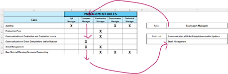
I've got close a few times with this but just can't nail it... I am wanting to populate sheets for staff that pull through their relevant job tasks based on: their job title as named in a column, and an 'X' where it applies to them. However, I want to extract the task name, not the 'X' itself, so there's a slight adjust to the column reference required. I've tried Index/Match, Filter and some other combinations, but can't quite get that sweet spot! Could anyone please guide me on this? Thanks

 

[MichaelLFC96]

=INDEX($B$2:$AA$2,SUMPRODUCT(MAX(($B$4:$AA$69=B103)*(COLUMN($B$4:$AA$69))))-COLUMN(B35)+1)

I use this on my sheet to extract column and row headers, I'm not sure if you can adjust where appropriate or it may open some doors for you to amend where you see fit.

Not sure how it would work for x in a box as they are all matching data and excel wouldn't be able to define each instance

 

[Eduard_Stoo]

Thanks, I've given it a go but can't quite get it singing...

The "X" should trigger a check against the value in Column A, which is unique so should mean you can make unique references to the left?

 

[Fluff]

Hi & welcome to MrExcel.
How about

=FILTER(A3:A100,CHOOSECOLS(C3:G100,XMATCH(J3,C3:G3))="x")

 

[Special-K99]

I had

=IFERROR(INDEX($A$3:A$8,AGGREGATE(15,6,ROW($A$3:$A$8)/(INDIRECT("$"&MID("CDEFG",MATCH($J$3,$C$2:$J$2,0),1)&"$3:$"&MID("CDEFG",MATCH($J$3,$C$2:$J$2,0),1)&"$8")="x"),ROWS($A$3:A3))-(3-1),COLUMNS($A1:A1)),"")

 

[Eduard_Stoo]

Thanks, got that working - I had to XMATCH to C2:G2 not C3:G3 as it's matching the header name, hope that's right. It only works as an array formula too, I think that's how the FILTER formula works if memory serves...

 

[Fluff]

It only works as an array formula too

If by that you mean using Ctrl Shift Enter, then don't. There is no need to do that for any formula in 365.

 

[Eduard_Stoo]

Thanks Fluff - I am actually fetching this data from another tab. If I just use the formula as standard it just 'SPILL!'s and doesn't populate, however if I array it, it works just fine?

It is actually in this form, and the real sheet is much larger.
=IFERROR(FILTER('Training Record Tasks List'!C3:C104,CHOOSECOLS('Training Record Tasks List'!$E$3:$AE$104,XMATCH($AB$1,'Training Record Tasks List'!$E$2:$AE$2))="X"),""). I've had to mess with some of the 'absolute references' in places, otherwise it only pulls through one entry, or doesn't work, or spills. This combination works OK though!!

 

[Fluff]

Do NOT use Ctrl Shift Enter.
Clear all the cells below the formula & enter it normally.