Dynamic Named Range based on values in multiple columns

[spence524]

Is there way to create a dynamic named range based on cell values from other columns? The cells in the named range may not be contiguous.
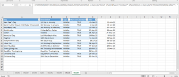
For example, I have a list of holidays or other observed days. I want a dynamic named range of the Day column to reference only those marked as Type: Holiday, and Mark on Calendar = TRUE.
If I remember, there was a combination of OFFSET and perhaps INDEX/MATCH. I've been searching other forums and pages and have not been able to find the solution.

 

[Jeffrey Mahoney]

What are you trying to return? The date or the Holiday description?

I would create a helper column that tests the Type and Mark on Calendar:
=IF(AND(B2="Holiday",C2=True),D2,"")
This puts a date in column E only if Holiday and Mark are true.

 

[spence524]

What are you trying to return? The date or the Holiday description?

I would create a helper column that tests the Type and Mark on Calendar:
=IF(AND(B2="Holiday",C2=True),D2,"")
This puts a date in column E only if Holiday and Mark are true.

The Date.
So the named range would end up having {1/1/23;1/16/23;2/20/23......} and so on.
Ahh, a helper column sounds like a great idea to help with the multiple conditions. Great idea!

 

[Jeffrey Mahoney]

Then you can use the FILTER function to return the dates from the new helper column

 

[Jeffrey Mahoney]

You should update your profile so we can see what version of MS Office and Operating system being used.

 

[spence524]

Then you can use the FILTER function to return the dates from the new helper column

I can use the FILTER function, but other users may not be able to.

 

[Jeffrey Mahoney]

Provide data instead of a picture. I can create a function that doesn't use FILTER

 

[spence524]

Provide data instead of a picture. I can create a function that doesn't use FILTER

 

[spence524]

I would like to be able to take the dates that are in bold and have that be a dynamic named range based on the helper column F. Currently, I have manually named the range for clarity. Thanks for looking at this!

Book1
	A	B	C	D	E	F
1	Day	Description	Type	Mark on Calendar?	Date	h_ActiveHoliday
2	New Year's Day	1st Day in January	Holiday	TRUE	1/1/2023	TRUE
3	Martin Luther King Jr.'s Birthday (Observed)	3rd Monday in January	Holiday	TRUE	1/16/2023	TRUE
4	Presidents Day	3rd Monday in February	Holiday		2/20/2023	FALSE
5	Good Friday	Friday Before Easter	Holiday	TRUE	4/7/2023	TRUE
6	Easter	Volatile	Holiday	TRUE	4/9/2023	TRUE
7	Memorial Day	Last Monday in May	Holiday	TRUE	5/29/2023	TRUE
8	Flag Day	14th Day in June	Holiday		6/14/2023	FALSE
9	Independence Day	4th Day in July	Holiday	TRUE	7/4/2023	TRUE
10	Labor Day	1st Monday in September	Holiday	TRUE	9/4/2023	TRUE
11	Columbus Day	2nd Monday in October	Holiday	TRUE	10/9/2023	TRUE
12	Thanksgiving Day	4th Thursday in November	Holiday	TRUE	11/23/2023	TRUE
13	Day After Thanksgiving	Day After Thanksgiving	Holiday		11/24/2023	FALSE
14	Christmas Eve	Day before Christmas	Holiday	TRUE	12/24/2023	TRUE
15	Christmas Day	25th Day in December	Holiday	TRUE	12/25/2023	TRUE
Sheet1

Cell Formulas
Range	Formula
E2	E2	=DATE(YEAR(NOW()),1,1)
F2:F15	F2	=AND([@Type]="Holiday",[@[Mark on Calendar?]]=TRUE)
E3	E3	=DATE(YEAR(NOW()),1,1)+IF(2<WEEKDAY(DATE(YEAR(NOW()),1,1)),7-WEEKDAY(DATE(YEAR(NOW()),1,1))+2,2-WEEKDAY(DATE(YEAR(NOW()),1,1)))+((3-1)*7)
E4	E4	=DATE(YEAR(NOW()),2,1)+IF(2<WEEKDAY(DATE(YEAR(NOW()),2,1)),7-WEEKDAY(DATE(YEAR(NOW()),2,1))+2,2-WEEKDAY(DATE(YEAR(NOW()),2,1)))+((3-1)*7)
E5	E5	=(DOLLAR(("4/"&YEAR(NOW()))/7+MOD(19*MOD(YEAR(NOW()),19)-7,30)*14%,)*7-6)-2
E6	E6	=DOLLAR(("4/"&YEAR(NOW()))/7+MOD(19*MOD(YEAR(NOW()),19)-7,30)*14%,)*7-6
E7	E7	=DATE(YEAR(NOW()),6,1)+IF(2<WEEKDAY(DATE(YEAR(NOW()),6,1)),7-WEEKDAY(DATE(YEAR(NOW()),6,1))+2,2-WEEKDAY(DATE(YEAR(NOW()),6,1)))+((1-1)*7)-7
E8	E8	=DATE(YEAR(NOW()),6,14)
E9	E9	=DATE(YEAR(NOW()),7,4)
E10	E10	=DATE(YEAR(NOW()),9,1)+IF(2<WEEKDAY(DATE(YEAR(NOW()),9,1)),7-WEEKDAY(DATE(YEAR(NOW()),9,1))+2,2-WEEKDAY(DATE(YEAR(NOW()),9,1)))+((1-1)*7)
E11	E11	=DATE(YEAR(NOW()),10,1)+IF(2<WEEKDAY(DATE(YEAR(NOW()),10,1)),7-WEEKDAY(DATE(YEAR(NOW()),10,1))+2,2-WEEKDAY(DATE(YEAR(NOW()),10,1)))+((2-1)*7)
E12	E12	=DATE(YEAR(NOW()),11,1)+IF(5<WEEKDAY(DATE(YEAR(NOW()),11,1)),7-WEEKDAY(DATE(YEAR(NOW()),11,1))+5,5-WEEKDAY(DATE(YEAR(NOW()),11,1)))+((4-1)*7)
E13	E13	=DATE(YEAR(NOW()),11,1)+IF(5<WEEKDAY(DATE(YEAR(NOW()),11,1)),7-WEEKDAY(DATE(YEAR(NOW()),11,1))+5,5-WEEKDAY(DATE(YEAR(NOW()),11,1)))+((4-1)*7)+1
E14	E14	=DATE(YEAR(NOW()),12,24)
E15	E15	=DATE(YEAR(NOW()),12,25)

Cells with Data Validation
Cell	Allow	Criteria
D2:D15	List	True, False

 

[shinigamilight]

G2: =IFERROR(INDEX(Table5[Date],AGGREGATE(15,6,(ROW(Table5[Mark on Calendar?])-1)/(--(Table5[Type]="Holiday")*--(Table5[Mark on Calendar?]=TRUE)),ROWS($G$2:G2))),"")


Maybe something like this?