MrAStanley
New Member
- Joined
- Dec 20, 2021
- Messages
- 2
- Office Version
- 365
- 2021
- 2019
- Platform
- Windows
Hi Guys,
I am really hoping somebody can help me with this as I have tried everything but still cannot find a viable solution.
My goal is to be able to identify overlapping mileage (miles and yards) from within my excel file.
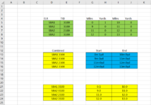
Please see below an example of the data...

(Please ignore the ELR and TID values for now)
I would like to be able to "flag up" rows which have overlapping mileage. As you can see, one start value would be 'Miles' and 'Yards' together (0.1) and the end would also be 'Miles' and 'Yards' together (10.0).
I figured that a Concatenate formula would get these together to form a more manageable value which is fine. However, I simply cannot find a solution to the initial problem of being able identify the overlapping data ranges.
We have an overlap here in the first 2 rows, as 9.0 - 11.0 also overlaps with the row above 0.1 - 10.0. This is one mile of overlap.
Another example image which may better explain the overlap issue can be seen here...

Is there is formula that can be used to achieve this outcome? I've never really been any good at Excel so I'm really hoping that an expert here can help me out.
Hopefully this all makes sense. The ELR and TID we can check by eye at this stage, I just need to get the overlapping mileages to highlight, in order to avoid overlapping sections.
Thank you in advance.
Andrew.
I am really hoping somebody can help me with this as I have tried everything but still cannot find a viable solution.
My goal is to be able to identify overlapping mileage (miles and yards) from within my excel file.
Please see below an example of the data...
(Please ignore the ELR and TID values for now)
I would like to be able to "flag up" rows which have overlapping mileage. As you can see, one start value would be 'Miles' and 'Yards' together (0.1) and the end would also be 'Miles' and 'Yards' together (10.0).
I figured that a Concatenate formula would get these together to form a more manageable value which is fine. However, I simply cannot find a solution to the initial problem of being able identify the overlapping data ranges.
We have an overlap here in the first 2 rows, as 9.0 - 11.0 also overlaps with the row above 0.1 - 10.0. This is one mile of overlap.
Another example image which may better explain the overlap issue can be seen here...
Is there is formula that can be used to achieve this outcome? I've never really been any good at Excel so I'm really hoping that an expert here can help me out.
Hopefully this all makes sense. The ELR and TID we can check by eye at this stage, I just need to get the overlapping mileages to highlight, in order to avoid overlapping sections.
Thank you in advance.
Andrew.
") We just need to identify these overlaps by any means necessary at this point.
We just need to identify these overlaps by any means necessary at this point.