Finding consecutive date pattern

[ronie85]

Hi

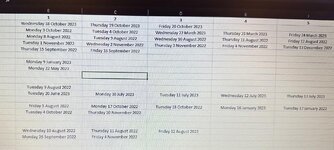
I require a formula that checks dates shown on a row and sees if they are consecutive days, and return the quantity of consecutive days.

If possible it also needs to discard weekend days, therefore Thursday 1st, Friday 2nd and Monday 5th will count as 3 consecutive days.

Finally, each row will contain a lot a few different consecutive sequences therefore the formula will need to find the 1st sequence, 2nd sequence and so on. Each sequence will count as an individual period.

 

[KRice]

...and return the quantity of consecutive days.

Could you clarify what results you expect? For each row, are you interested in a summary of the number of consecutive date periods, the number of dates in each of those periods, or the actual periods described in terms of their start and end dates. For example, for...

MrExcel_20231210.xlsx
	B	C	D	E	F	G
3	Mon, 10/3/22	Tue, 10/4/22	Wed, 3/22/23	Thu, 3/23/23	Fri, 3/24/23	Thu, 4/13/23
Sheet1

do you want:

1. 2 consecutive date periods
2. 2 consecutive date periods consisting of one 2-day period and one 3-day period
3. 10/3/22-10/4/22, 3/22/23-3/24/23
4. something else

 

[ronie85]

Ideally I would like 3 things.
1) Number of different periods which could be 1 day or more. If the days are consecutive, they will be classed as a period
2) The length of each period in days (excluding weekend days). If needed, I could setup a range of dates and exclude all of the weekend days so that the formula is solely looking for unbroken dates.
3) The start and end date of each period

 

[ronie85]

I made a date range excluding weekend days if that helps

 

[KRice]

Thank you. I understand the content of the desired output, but I am not sure about the desired output structure and format. Please have a look at this. For each row, I've left the four supporting formulas separate:

1. The green-shaded region creates an array that maps the dates in the original array to a group number, where a group is defined as all dates within a period of contiguous workdays
2. The red-shaded region describes the number of periods of contiguous workdays
3. The blue-shaded region describes the number of days within each period of contiguous workdays (in separate columns)
4. The yellow-shaded region describes the date ranges of each period of contiguous workdays (in separate columns)

You could use this "as is" and hide the "helper" array (green-shaded region), or the formula that creates the green-shaded region could be incorporated into the other formulas. Also, the red, blue, and yellow outputs could be combined so that all results "spill" from a single formula, but the array lengths for each of these are likely different as we move from row to row, so the output arrays would need to be padded with blanks so that the final outputs are properly aligned.

MrExcel_20231210.xlsx
	B	C	D	E	F	G	H	I	J	K	L	M	N	O	P	Q	R	S	T	U	V
11	1	2	3	4	5	6		Nperiods	Length of Periods			Dates of Periods
12	Wed, 10/18/23	Thu, 10/19/23	Fri, 10/20/23					1	3			18/10/2023-20/10/2023				1	1	1
13	Mon, 10/3/22	Tue, 10/4/22	Wed, 3/22/23	Thu, 3/23/23	Fri, 3/24/23	Thu, 4/13/23		3	2	3	1	03/10/2022-04/10/2022	22/03/2023-24/03/2023	13/04/2023		1	1	2	2	2	3
14	Mon, 8/8/22	Tue, 8/9/22	Wed, 8/10/22	Thu, 8/11/22	Fri, 8/12/22			1	5			08/08/2022-12/08/2022				1	1	1	1	1
15	Tue, 6/20/23	Mon, 7/10/23	Tue, 7/11/23	Wed, 7/12/23				2	1	3		20/06/2023	10/07/2023-12/07/2023			1	2	2	2
16	Fri, 10/14/22	Mon, 10/17/22	Tue, 10/18/22	Mon, 1/16/23	Tue, 1/17/23			2	3	2		14/10/2022-18/10/2022	16/01/2023-17/01/2023			1	1	1	2	2
Sheet1

Cell Formulas
Range	Formula
I12:I16	I12	=MAX(Q12#)
J12,J14,J15:K16,J13:L13	J12	=COUNTIF(Q12#,SEQUENCE(,MAX(Q12#)))
M12,M14,M15:N16,M13:O13	M12	=LET(rng,B12:G12,seq,SEQUENCE(,MAX(Q12#)),first,XMATCH(seq,Q12#,0,1),last,XMATCH(seq,Q12#,0,-1),BYCOL(seq,LAMBDA(x,IF(INDEX(first,,x)=INDEX(last,,x),TEXT(INDEX(rng,,INDEX(first,,x)),"dd/mm/yyyy"),TEXTJOIN("-",,TEXT(INDEX(rng,,INDEX(first,,x)),"dd/mm/yyyy"),TEXT(INDEX(rng,,INDEX(last,,x)),"dd/mm/yyyy"))))))
Q12:S12,Q16:U16,Q15:T15,Q14:U14,Q13:V13	Q12	=LET(rng,B12:G12,TRANSPOSE(SCAN(1,SEQUENCE(COUNT(rng)),LAMBDA(a,v,IF(v=1,1,IF(NETWORKDAYS(INDEX(rng,,v-1),INDEX(rng,,v))-1=1,a,a+1))))))
Dynamic array formulas.

 

[KRice]

Here is a similar version with the formulas combined into a single, multi-part formula that determines the three outputs (number of periods, length of each period, date range of each period) and then combines them into a single spilled array. To avoid confusion, each of these sub-parts needs to be the same length, so the user needs to specify the maximum number of contiguous periods that might be encountered on the worksheet (in this example I set the variable maxn=4, meaning that the array describing the length (in days) of each of the contiguous workday periods is padded to produce an array consisting of 4 items). Similarly, the array describing the date ranges of contiguous workday periods is also padded to produce an array of 4 elements. To use the formula, specify the range for the row of dates (a variable I've named rng) based on specifying the leftmost cell in the range and the rightmost cell in the data table of dates (it is okay if this produces a formulas whose "rng" includes blanks in the rightmost cells, as these will be ignored by the formula). The formula, can then be copied down beside the date data table. It is possible (I think) to avoid needing to specify maxn, but that would require constructing the helper array "pds" so that it spills in two directions, both down the length of the table and across so that the maximum output array size could be determined, and then that value would be taken as maxn. This would add substantial complexity to the formula, so if manually setting maxn is satisfactory, I would recommend avoiding further complications. If you discover that a row does not have sufficient space to accommodate the spilled results (indicated by a SPILL error), simply increase the value of maxn and recopy the formula down the output section of the worksheet.

You may see that I changed the computation of the array called "lpds" (the length in days of each contiguous workday period), as this single-formula approach requires referencing the array called "pds" rather than the range of spilled results shown in the previous post (in Q12#), and COUNTIF used previously does not accept an array as an argument...so I've generated the lpds array using a different method (with the FREQUENCY function and then transformed the output to be compatible with the other results).

MrExcel_20231210.xlsx
	B	C	D	E	F	G	H	I	J	K	L	M	N	O	P	Q
19	1	2	3	4	5	6		Nperiods	Length of Periods				Dates of Periods
20	Wed, 10/18/23	Thu, 10/19/23	Fri, 10/20/23					1	3				18/10/2023-20/10/2023
21	Mon, 10/3/22	Tue, 10/4/22	Wed, 3/22/23	Thu, 3/23/23	Fri, 3/24/23	Thu, 4/13/23		3	2	3	1		03/10/2022-04/10/2022	22/03/2023-24/03/2023	13/04/2023
22	Mon, 8/8/22	Tue, 8/9/22	Wed, 8/10/22	Thu, 8/11/22	Fri, 8/12/22			1	5				08/08/2022-12/08/2022
23	Tue, 6/20/23	Mon, 7/10/23	Tue, 7/11/23	Wed, 7/12/23				2	1	3			20/06/2023	10/07/2023-12/07/2023
24	Fri, 10/14/22	Mon, 10/17/22	Tue, 10/18/22	Mon, 1/16/23	Tue, 1/17/23			2	3	2			14/10/2022-18/10/2022	16/01/2023-17/01/2023
Sheet1

Cell Formulas
Range	Formula
I20:Q24	I20	=LET(rng,B20:G20,maxn,4, pds,TRANSPOSE(SCAN(1,SEQUENCE(COUNT(rng)),LAMBDA(a,v,IF(v=1,1,IF(NETWORKDAYS(INDEX(rng,,v-1),INDEX(rng,,v))-1=1,a,a+1))))), npds,MAX(pds), lpds,TRANSPOSE(DROP(FREQUENCY(pds,SEQUENCE(,MAX(pds))),-1)), dpds,LET(seq,SEQUENCE(,MAX(pds)),first,XMATCH(seq,pds,0,1),last,XMATCH(seq,pds,0,-1),BYCOL(seq,LAMBDA(x,IF(INDEX(first,,x)=INDEX(last,,x),TEXT(INDEX(rng,,INDEX(first,,x)),"dd/mm/yyyy"),TEXTJOIN("-",,TEXT(INDEX(rng,,INDEX(first,,x)),"dd/mm/yyyy"),TEXT(INDEX(rng,,INDEX(last,,x)),"dd/mm/yyyy")))))), HSTACK(npds,EXPAND(lpds,1,maxn,""),EXPAND(dpds,1,maxn,"")))
Dynamic array formulas.

 

[ronie85]

Thank you. I understand the content of the desired output, but I am not sure about the desired output structure and format. Please have a look at this. For each row, I've left the four supporting formulas separate:

1. The green-shaded region creates an array that maps the dates in the original array to a group number, where a group is defined as all dates within a period of contiguous workdays
2. The red-shaded region describes the number of periods of contiguous workdays
3. The blue-shaded region describes the number of days within each period of contiguous workdays (in separate columns)
4. The yellow-shaded region describes the date ranges of each period of contiguous workdays (in separate columns)

You could use this "as is" and hide the "helper" array (green-shaded region), or the formula that creates the green-shaded region could be incorporated into the other formulas. Also, the red, blue, and yellow outputs could be combined so that all results "spill" from a single formula, but the array lengths for each of these are likely different as we move from row to row, so the output arrays would need to be padded with blanks so that the final outputs are properly aligned.

MrExcel_20231210.xlsx
	B	C	D	E	F	G	H	I	J	K	L	M	N	O	P	Q	R	S	T	U	V
11	1	2	3	4	5	6		Nperiods	Length of Periods			Dates of Periods
12	Wed, 10/18/23	Thu, 10/19/23	Fri, 10/20/23					1	3			18/10/2023-20/10/2023				1	1	1
13	Mon, 10/3/22	Tue, 10/4/22	Wed, 3/22/23	Thu, 3/23/23	Fri, 3/24/23	Thu, 4/13/23		3	2	3	1	03/10/2022-04/10/2022	22/03/2023-24/03/2023	13/04/2023		1	1	2	2	2	3
14	Mon, 8/8/22	Tue, 8/9/22	Wed, 8/10/22	Thu, 8/11/22	Fri, 8/12/22			1	5			08/08/2022-12/08/2022				1	1	1	1	1
15	Tue, 6/20/23	Mon, 7/10/23	Tue, 7/11/23	Wed, 7/12/23				2	1	3		20/06/2023	10/07/2023-12/07/2023			1	2	2	2
16	Fri, 10/14/22	Mon, 10/17/22	Tue, 10/18/22	Mon, 1/16/23	Tue, 1/17/23			2	3	2		14/10/2022-18/10/2022	16/01/2023-17/01/2023			1	1	1	2	2
Sheet1

Cell Formulas
Range	Formula
I12:I16	I12	=MAX(Q12#)
J12,J14,J15:K16,J13:L13	J12	=COUNTIF(Q12#,SEQUENCE(,MAX(Q12#)))
M12,M14,M15:N16,M13:O13	M12	=LET(rng,B12:G12,seq,SEQUENCE(,MAX(Q12#)),first,XMATCH(seq,Q12#,0,1),last,XMATCH(seq,Q12#,0,-1),BYCOL(seq,LAMBDA(x,IF(INDEX(first,,x)=INDEX(last,,x),TEXT(INDEX(rng,,INDEX(first,,x)),"dd/mm/yyyy"),TEXTJOIN("-",,TEXT(INDEX(rng,,INDEX(first,,x)),"dd/mm/yyyy"),TEXT(INDEX(rng,,INDEX(last,,x)),"dd/mm/yyyy"))))))
Q12:S12,Q16:U16,Q15:T15,Q14:U14,Q13:V13	Q12	=LET(rng,B12:G12,TRANSPOSE(SCAN(1,SEQUENCE(COUNT(rng)),LAMBDA(a,v,IF(v=1,1,IF(NETWORKDAYS(INDEX(rng,,v-1),INDEX(rng,,v))-1=1,a,a+1))))))
Dynamic array formulas.

I have only got around to implimenting this today and it is amazing! More data than I required and I am using it all!

 

[ronie85]

Thank you very much!

 

[KRice]

That's great to hear...thanks for the update! I'm happy to help.