Additional question: What is your Office version? (You can set this information
in your account to let helpers to know your Office version and platform, so they can provide compatible solutions).
For Office 365, we can use
UNIQUE and
SORT functions (available in 365) to create a data validation list. Here how I set it up in my worksheet for the same data structure in the original question.
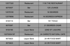
I wrote the following formula in cell K1.
Excel Formula:
=SORT(UNIQUE(OFFSET($C$1,1,,COUNTA($C:$C)-1,1)))
This creates a unique list of business names in the column C as shown below. Since UNIQUE and SORT are spilling functions, the list goes down as much as necessary.
View attachment 26456
Then I selected cell L1, and created a List data validation with the following formula:
View attachment 26457
So, this is the result:
View attachment 26458
You can preferably hide the column K.
Now, the Conditional Formatting step.
I selected A1 cell in the worksheet again, then I clicked on Conditional Formatting->Manage Rules->New Rule, and selected the "Use a formula to determine which cells to format" option. Selected Format, and set the Font as Strikethrough.
Then I entered the following formula in the "Format values where this formula is true" text box. This is basically checking if cell is not blank, and matches the current cell value with the currently selected business name in cell L1. This is also matching the first 5 chars as I assume you still need this here as well. If full match is required, then the formula could be updated by removing the
LEFT function.
Excel Formula:
=AND(NOT(ISBLANK($C1)), LEFT($C1,5) = LEFT($L$1,5))
Clicked OK, and the new rule is in the list with the previous rule I created. I changed the "Applies to" field to be "$A:$I", and clicked OK.
View attachment 26461
And I got all the rows matching with the selected business name (first 5 chars) in cell L1 as strikethrough as show below, previous conditional formatting rule is also applied:
View attachment 26462
Hope this helps.