I'm using =SUMIFS($D$18:$D$33,$B$18:$B$33,B4) which works well, but I need the formula to read only the first 4 digits in the sum range of $D$18:$D$33 then have those first 4 digits that match what is in B4 so that it can return the sum of the criteria range $B$18:$B$33. Can this be done? (The data in the cells will be changing each month, so each month I will edit the 4 digits in B4 and need to have the first 4 digits of the sum range match what is in B4.) Can this be done? Thanks in advance!
-
If you would like to post, please check out the MrExcel Message Board FAQ and register here. If you forgot your password, you can reset your password.
You are using an out of date browser. It may not display this or other websites correctly.
You should upgrade or use an alternative browser.
You should upgrade or use an alternative browser.
Formula =SUMIF for a sum range of the first 4 digits only in the cells
- Thread starter schrieber
- Start date
Excel Facts
Does the VLOOKUP table have to be sorted?
No! when you are using an exact match, the VLOOKUP table can be in any order. Best-selling items at the top is actually the best.
kweaver
Well-known Member
- Joined
- May 12, 2009
- Messages
- 2,934
- Office Version
- 365
- 2010
How about:
| SampleText.txt | |||||
|---|---|---|---|---|---|
| B | C | D | |||
| 3 | Project # | Project # | |||
| 4 | 4311 | 3637 | |||
| 5 | Total Hours: | Total Hours: | |||
| 6 | 6.5 | 22.5 | |||
| 7 | |||||
| 8 | |||||
| 9 | |||||
| 10 | |||||
| 11 | |||||
| 12 | |||||
| 13 | |||||
| 14 | |||||
| 15 | |||||
| 16 | |||||
| 17 | Project Name | Type | Project Hours | ||
| 18 | 4311-GENERIC.00 | HB | 6.5 | ||
| 19 | 9999-ADMIN.00 | NB | 1.0 | ||
| 20 | 3637-ALPHA | PB | 1.5 | ||
| 21 | 3637-MAIN | PB | 21.0 | ||
| 22 | |||||
| 23 | |||||
| 24 | |||||
| 25 | |||||
Sheet3 | |||||
| Cell Formulas | ||
|---|---|---|
| Range | Formula | |
| B6:C6 | B6 | =SUM(IFERROR(B4=1*LEFT($B$18:$B$25,4),0)*$D$18:$D$25) |
Upvote
0
Yes that works - thanks!How about:
SampleText.txt
B C D 3 Project # Project # 4 4311 3637 5 Total Hours: Total Hours: 6 6.5 22.5 7 8 9 10 11 12 13 14 15 16 17 Project Name Type Project Hours 18 4311-GENERIC.00 HB 6.5 19 9999-ADMIN.00 NB 1.0 20 3637-ALPHA PB 1.5 21 3637-MAIN PB 21.0 22 23 24 25
Cell Formulas Range Formula B6:C6 B6 =SUM(IFERROR(B4=1*LEFT($B$18:$B$25,4),0)*$D$18:$D$25)
Upvote
0
Your =SUM((--(ISNUMBER(FIND(B$4,$B$9:$B$19))))*($D$9:$D$19)) works great. When the 4 digit number is not found in B4, it returns a 0, which is great, but 1 question: Let's say next month, B4 is blank-- can the formula return a 0 if B4 is blank? (since my cell data changes each month). Currently, it returns the sum of all of ($D$9:$D$19)) when B4 is blank.Thanks for the table data. Try this:
Book1
A B C D E 1 2 3 Project # Project # 4 4311 3637 5 Total Hours: Total Hours: 6 6.5 22.5 Example: Need formula in B6 to return the total hours of the project # in B4 which resides in range B$18:$B$23, with the sum range of $D$18:$D$23 (So the total in B6 would be 6.5) 7 8 Project Name Type Project Hours 9 4311-GENERIC.00 HB 6.5 10 9999-ADMIN.00 NB 1 11 3637-ALPHA PB 1.5 12 3637-MAIN PB 21
Cell Formulas Range Formula B6:C6 B6 =SUM((--(ISNUMBER(FIND(B$4,$B$9:$B$12))))*($D$9:$D$12))
Upvote
0
My suggestion would be to display blank with this formula:
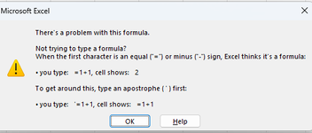
Excel Formula:=IF(B4="","",=SUM((--(ISNUMBER(FIND(B$4,$B$9:$B$19))))*($D$9:$D$19)))
Upvote
0
Perfection! Thanks to you both!Remove the = sign from infront of SUM
Upvote
0
Similar threads
- Replies
- 4
- Views
- 178
- Replies
- 1
- Views
- 392
- Replies
- 19
- Views
- 309
- Replies
- 7
- Views
- 162


