Formula to determine max number in multiple dynamic arrays

[jberylec]

This one is proving tough for me! Hope the experts can help

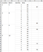
I need to create a formula in F2 that can be copied down through hundreds of location/batch rows, on a new version of this spreadsheet each day. The formula needs to find the max number in D but only for each location/batch section and report only that one into F on the same row. I've manually typed them in F just for display purposes.

A and B rows are always merged for that entire location and batch, as shown. So I was trying to build a formula that would recognize each time a row in B isn't blank <>"" which indicates a new location/batch starts here, then include that row and all blank rows below it (they're merged so treated as blank cells) to find the MAX number in D and show that in F. Then of course it starts over IF B isnt blank again.

In case of a tie, show both.

FYI, there are a lot more columns of data, not relevant for this though because none can be used as an identifier, I also have many other formula columns that I paste into row 2 each morning, then drag them all down the entire sheet, so trying to keep this just a formula not VBA. Hoping to add this new column to my daily paste and drag routine. Ah. Exhausting just describing this. Ha! Thanks in advance

 

[Peter_SSs]

.. the formula popup I talked about in post #4 and included a screenshot.

Ah, I see now. You can turn off 'Allow editing directly in cells' via File - Options -Advanced as shown below. You then edit in the formula bar instead. (I always have that setting off)

 

[jberylec]

Is there a small change possible for the INFA formula in column H to treat blanks in D as lowest instead of highest? All else seems to working very good Thanks in advance!

 

[Peter_SSs]

Try

=IF(D2="","",IFNA(MATCH(COUNTIFS(E$2:E$1000,E2,D$2:D$1000,">"&D2)+1,{1,2,3},0),""))

 

[jberylec]

Hi again Peter, yes thats how I was doing it, but the problem is that just hides the result instead of excluding it from taking up the 1st spot. So the remaining results are inaccurate because it only show 2nd highest and 3rd highest, because the 1st highest was simply just hidden by the "". If there's a way to instead throw a third criteria in the match or count? Something like D2<>""

Also, I'm using this brilliant formula in reverse in other areas to find the lowest numbers per location by switching the ">" to "<", which works great! But having a similar issue where I have zeros in the data and it treats 0 as the lowest, which is technically true, but I need to somehow ignore those. So if there's a solution to the above issue, like an additional criteria, then I can use that same solution to ignore zeros here too...

Many thanks my friend!

 

[Peter_SSs]

Hi again Peter, yes thats how I was doing it, but the problem is that just hides the result instead of excluding it from taking up the 1st spot. So the remaining results are inaccurate because it only show 2nd highest and 3rd highest, because the 1st highest was simply just hidden by the "".

Perhaps I am not understanding what you are saying but I don't believe that I am getting what you describe.
For the sample data below, which results are incorrect in columns G or H?

Otherwise, can you provide some XL2BB sample data that demonstrates the problem?

jberylec.xlsm
	A			D	E	F	G	H
1	Location			Max		Max	Top3	Top3
2	1			86	1		86	2
3				87	1	87	87	1
4				84	1		84	3
5					1
6	2			77	2		77	2
7				71	2
8					2
9					2
10				74	2		74	3
11				81	2	81	81	1
12	1			97	3		97	2
13				0	3
14				98	3	98	98	1
15				90	3
16				95	3		95	3
17	4			62	4		62	3
18					4
19					4
20					4
21					4
22					4
23				67	4		67	2
24				70	4	70	70	1
Max per group (3)

Cell Formulas
Range	Formula
E2:E24	E2	=E1+(A2<>"")
F2:F24	F2	=IF(D2=MAXIFS(D$2:D$1000,E$2:E$1000,E2),D2,"")
G2:G24	G2	=IF(D2>=AGGREGATE(14,6,D$2:D$1000/(E$2:E$1000=E2),3),D2,"")
H2:H24	H2	=IF(D2="","",IFNA(MATCH(COUNTIFS(E$2:E$1000,E2,D$2:D$1000,">"&D2)+1,{1,2,3},0),""))

 

[jberylec]

In the live spreadsheet, D is a formula with a string of IFs, the final value when false is ""
Example (but much longer formula): IF(this>that,this,"")

When D results in "" the IFNA in both G and H are treating it as the max value in range D. I cant think of a way to paste the XL2BB without including a bunch of columns that the formula in D references.

In short, if the D cell is actually blank, like in the above XL2BB example, or if I delete the formula from the cell, then IFNA is behaving correctly, but if its blank as in the resulting "" value from the IF formula then IFNA is treating it as text or something else greater than the actual numbers in the rest of the D range.

So, to get around that, instead of using "" as my final value when false, I changed it to zero, for example: IF(this>that,this,0)
But this introduces the second problem I was referring to where these zeros are now reported as my smallest value in the range, rather than the actual smallest I'm looking for. So I'd rather keep the "" but have it treated as a blank, not the max value.

Sorry if I'm not making sense

 

[Peter_SSs]

When D results in "" the IFNA in both G and H are treating it as the max value in range D.

Not for me.

jberylec.xlsm
	A			D	E	F	G	H	I	J	K
1	Location			Max		Max	Top3	Top3
2	1			86	1		86	2			86
3				87	1	87	87	1			87
4				84	1		84	3			84
5					1
6	2			77	2		77	2			77
7				71	2						71
8					2
9					2
10				74	2		74	3			74
11				81	2	81	81	1			81
12	1			97	3		97	2			97
13					3						0
14				98	3	98	98	1			98
15				90	3						90
16				95	3		95	3			95
17	4			62	4		62	3			62
18					4
19					4
20					4
21					4
22					4
23				67	4		67	2			67
24				70	4	70	70	1			70
Max per group (3)

Cell Formulas
Range	Formula
D2:D24	D2	=IF(K2,K2,"")
E2:E24	E2	=E1+(A2<>"")
F2:F24	F2	=IF(D2=MAXIFS(D$2:D$1000,E$2:E$1000,E2),D2,"")
G2:G24	G2	=IF(D2>=AGGREGATE(14,6,D$2:D$1000/(E$2:E$1000=E2),3),D2,"")
H2:H24	H2	=IF(D2="","",IFNA(MATCH(COUNTIFS(E$2:E$1000,E2,D$2:D$1000,">"&D2)+1,{1,2,3},0),""))

Check your column D formula. I suspect that instead of
IF(this>that,this,"")
I think that you may have this
IF(this>that,this," ")

 

[jberylec]

Yes I see it working in yours. But not mine. Its not a space in the "", checked that long ago. The only thing I can think of is maybe because my IF formula in D is much more complex than this simple example. For instance, mine starts with the blank, then moves on to check many things before giving the result, like this: IF(THIS,"",IF(AND(THAT,THIS),"",IF(YADA,"",IF(OR(YEAH,AND(YAH,NAH)),"", and finally if I get through these tests give me the number in K2 )))

The formulas all work well, other than their results are not being treated correctly by countifs and ifna, etc. I'll see if I can work up an example of this problem. Any way I can copy this sheet from the thread? I cant for the life of me find the original, I must've deleted. Bummer

Thanks again for all your help!

 

[Peter_SSs]

The length/complexity of the formula should make no difference as my formulas use the result of the formula only.
In blank cells in the sheet put these formulas and point them at one of the column D cells where the blanks are not being ignored. Report the results.

=LEN(D5)
=CODE(D5)

Any way I can copy this sheet from the thread?

You can copy my sheet to a blank worksheet by clicking this icon at the top left of my sheet, selecting A1 in your blank sheet, Paste.

Can you post a small section from your actual worksheet (first disguising any sensitive data and/or hiding any irrelevant columns/rows) with XL2BB?

 

[jberylec]

Ok I'll work on a live example, but its difficult because the cells referenced are spread out so far the XL2BB wont paste it all, and if I only grab the relevant section they all turn to #REF because the missing cells. So anyhow, for now until I mock up a new sheet, here's a screen snip of the live data.

This is an example of the second issue I was talking about in earlier posts, which could be just me misusing/modifying this formula. I changed the > to a < to try to get the lowest instead of the highest. Its counting blanks as the lowest. On the right you have the LEN, CODE, and the IFNA. They're all referencing the far left column, which in this case is column AZ, where the 62.50 should be the only 1 lowest, but you can see Excel is counting the blanks as the lowest also. I've triple checked the AZ cells, they are all resulting in "" because they all fail the IF formulas. All rows were copied down, so they're exactly the same formulas.

Here's the formula in the far right column: IFNA(MATCH(COUNTIFS(BF$2:BF$1500,BF112,AZ$2:AZ$1500,"<"&AZ112)+1,{1,2},0),""))

BF is our anchor column, they all have the same 14, and I've checked the entire spreadsheet for any weirdness, nope, this part of the range creation is working perfectly. There are no other 14's in the sheet.

I've tried removing the +1, and changing it to +0 and -1, each giving different results, but still not the expected, so perhaps I just butchered this formula to try to get the lowest 2.

Hopefully an easy fix/oversight on my part, but if not I'll of course keep working on a mock up file that fits inside the copy/paste limits and doesn't #REF out all the cells.

Also I'll keep scouring for an example of the other issue where the unaltered formula is considering the blanks as the highest/largest.

Thanks again!