Formula Help (Most likely Dynamic Array Needed)

[Magoosball]

Hello -- Please see image attached. I'm using Microsoft 365. Thank you!!

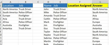
I'm looking to write a formula in the Location Assigned (Column F) that produces the results I manually inputted in the Answer (Column G)

Basically I have a list of Locations and Jobs in column A and B. I'm trying to assign each person in column D to the location where the least people are currently based off their job in column E.
For example: Caitlin is a police officer. Mike was already assigned to South America. Therefor the least amount of Police officers are currently assigned to Africa, which is 0.


I can use multiple helper columns if needed. When I was trying to do this previously I was receiving a circular reference error because when I dragged down the formula in the location assigned column each answer was dependent on the assignment made in the previous row.

thank you for your help and let me know if you have any questions!

 

[Fluff]

How about

=LET(f,FILTER($A$2:$A$8,$B$2:$B$8=E2),INDEX(f,MOD(COUNTIFS(E$2:E2,E2)-1,ROWS(f))+1))

 

[Magoosball]

How about

=LET(f,FILTER($A$2:$A$8,$B$2:$B$8=E2),INDEX(f,MOD(COUNTIFS(E$2:E2,E2)-1,ROWS(f))+1))

this worked perfectly - thank you!!!

 

[Fluff]

You're welcome & thanks for the feedback.

 

[Magoosball]

How about

=LET(f,FILTER($A$2:$A$8,$B$2:$B$8=E2),INDEX(f,MOD(COUNTIFS(E$2:E2,E2)-1,ROWS(f))+1))

Hi Fluff,

I have a slight modification and wondering if you could assist. See the attached Screenshot. Instead of assigning to the lowest location based off a count; I'd like to assign to The Lowest "Fill".

Column C is a value
Column D is

=COUNTIFS(I:I,A2,H:H,B2)

Column E =

=D2/C2

Basically i'm taking a current number assigned so far, dividing by an amount required, and assigning them to the lowest rate.

thank you!!

 

[Fluff]

What do you mean by the lowest fill?
Also please post your data using the Xl2BB add-in, rather than an image.

 

[Magoosball]

What do you mean by the lowest fill?
Also please post your data using the Xl2BB add-in, rather than an image.

I mean the lowest percentage in the rate column E. Xl2BB addin below:

Question.xlsx
	A	B	C	D	E	F	G	H	I	J	K	L
1	Location	Job	Needed	Assigned	Rate		Name	Job	Location Assigned	Answer
2	North America	Truck Driver	3	0	0%		John	Truck Driver		North America
3	South America	Police Officer	7	0	0%		Mike	Police Officer		South America
4	Europe	Firefighter	4	0	0%		Amanda	Truck Driver		Asia		Location Assigned formula in cell I2 should be the Location in column A that has the " Min Rate" in column E
5	Asia	Truck Driver	7	0	0%		Caitlin	Police Officer		Africa
6	Africa	Police Officer	4	0	0%		Mark	Firefighter		Europe
7	Australia	Firefighter	8	0	0%		Jim	Firefighter		Australia
8	Antartica	Truck Driver	19	0	0%		Gus	Truck Driver		Antartica
9							Taylor	Police Officer		South America
10							Haylee	Truck Driver		North America
11							Sabrina	Police Officer		Africa
12							Martin	Firefighter		Europe
13							Beth	Firefighter		Australia
Sheet1

Cell Formulas
Range	Formula
D2:D8	D2	=COUNTIFS(I:I,A2,H:H,B2)
E2:E8	E2	=D2/C2

 

[Fluff]

But the formula I supplied gives what you have shown for the expected results.

 

[Magoosball]

The result of I10 here in red should be Antartica because it has the lowest rate of Truck Drivers in column E of 5 %. There are 3 Truck Driver Locations, North America with a rate of 33%, Asia with a rate of 14% and Antartica with a rate of 5%. Antartica has the lowest rate of 5% so cell I10 should return Antartica. Currently the formula in cell I10 is returning North America

Question.xlsx
	A	B	C	D	E	F	G	H	I
1	Location	Job	Needed	Assigned	Rate		Name	Job	Location Assigned
2	North America	Truck Driver	3	1	33%		John	Truck Driver	North America
3	South America	Police Officer	7	2	29%		Mike	Police Officer	South America
4	Europe	Firefighter	4	1	25%		Amanda	Truck Driver	Asia
5	Asia	Truck Driver	7	1	14%		Caitlin	Police Officer	Africa
6	Africa	Police Officer	4	1	25%		Mark	Firefighter	Europe
7	Australia	Firefighter	8	1	13%		Jim	Firefighter	Australia
8	Antartica	Truck Driver	19	1	5%		Gus	Truck Driver	Antartica
9							Taylor	Police Officer	South America
10							Haylee	Truck Driver
11							Sabrina	Police Officer
12							Martin	Firefighter
13							Beth	Firefighter
Sheet1

Cell Formulas
Range	Formula
D2:D8	D2	=COUNTIFS(I:I,A2,H:H,B2)
E2:E8	E2	=D2/C2
I2:I9	I2	=LET(f,FILTER($A$2:$A$8,$B$2:$B$8=H2),INDEX(f,MOD(COUNTIFS(H$2:H2,H2)-1,ROWS(f))+1))

 

[Fluff]

Currently the formula in cell I10 is returning North America

That's because you originally said it should & also showed that as the correct answer in post#7. It's very difficult to help when you keep changing things.
As the formula in col D is looking at col I you are going to get a circular reference when using col E to determine what is in col I