How to avoid Circular Reference in specific example

[Magoosball]

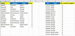
Yellow columns in image contain formulas

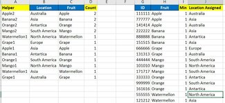
Column A Formula =C2&D2
Column D Formula =COUNTIFS(H:H,C2,J:J,B2)
Column I Formula =MINIFS(D:D,C:C,H2)

Column J Formula - Currently receiving a circular reference with this formula --- =XLOOKUP(H2&I2,A:A,B:B)

The result in each subsequent cell in column J is impacted by the prior cell in column J.

The overall objective of the formula in column J that I'm looking for is to write a formula that assigns the location that currently has the lowest count, or the fewest currently assigned to it.

Is there a way to write this in a way where I don't receive a circular reference error?

I'm on Excel 365.

thank you!

 

[Muhammad_Usman]

Why you use Colum JJ in Countifs function . I think if you remove it will working without error.


Column D Formula =COUNTIFS(H:H,C2,J:J,B2)

 

[Magoosball]

I'm trying to assign all the fruits in Column H a location with the formula written in column J.

The location I'm trying to assign them to is where the least amount of fruits of that specific type are currently assigned based off the previous fruits assigned in column J.

For example with no formula in column J, the count in column D is 0. The first apple should get assigned to Australia. Now that Australia has 1 apple the 2nd apple in column J should be assigned to Asia because it currently has the least amount of apples assigned to it. The third apple - the formula sees that there is 1 apple in Australia, 1 apple in Asia, so it assigns to Australia (the first in the list here.




One way I could think of creating this is with vba. where the script starts off calculating. Then copying and pasting columns A - D as values. Write the xlookup formula in column J. calculate. copy and paste column j as values. re write the formulas in column A - D. calculate. copy and paste as values --------- in an infinite loop until all rows in column J are assigned.

Is there a way to do the same thing without having to use VBA to paste them as values each time it re calculates? - I'd probably have to look at the array as a whole in order to do so?

the image attached here is what i'd expect the answer to be. these are values instead of a formula producing the result. I'd have to use a formula though just because the list can become thousands long